Spawning Phenology and Early Growth of Japanese Anchovy (Engraulis japonicus) off the Pacific Coast of Japan

Abstract

The reproduction and early growth of fish are essential elements that affect recruitment and provide breakthrough points for understanding population fluctuations. In this study, larval and juvenile Japanese anchovy (Engraulis japonicus) were collected from five coastal waters off the Pacific coast of Japan in 2020 and 2021 to gain more insight into life history traits such as reproduction and early growth of this species on the basis of otolith microstructure analysis. The spawning period appeared to be related to temperature and chlorophyll-a concentrations, showing latitudinal gradient variation among fishing areas. We detected a significant positive allometric growth pattern between standard length and body weight. The Gompertz model best fits the growth of standard length, showing an initial stage of growth that was quick and accelerating. The mean daily growth rate for standard length was 0.64 ± 0.09 mm per day. A series of mixed-effect models was constructed to investigate the sources of differences in the mean growth rates among individuals. The results revealed regional variability in fish growth, with individuals in the central Pacific stock growing faster. Individuals that grew slower were heavier than those of the same length, indicating a trade-off between length growth and weight growth. The mean growth of individual fish was positively influenced by environmental factors (surface water temperature and chlorophyll-a concentration), and individuals within the same school of fish displayed a striking homogeneity of growth. Our research demonstrates the significance of including both physiological characteristics and environmental influences in early growth studies on fish.

1. Introduction

Early life history of fish and its role in recruitment processes has given rise to successive studies in fisheries. The degree to which the timing and location of spawning match the environmental conditions required for larval development is critical for larval growth and survival [1,2]. Growth during the early stages is recognized as an essential determinant of recruitment success in fish populations [3,4], influencing fishery resource biomass, which is related to fisheries production [5,6,7]. Our knowledge of fish population fluctuations and changes in population structure relies on the knowledge of reproduction and early growth, which are closely related to mortality [8,9], especially for small pelagic fish characterized by high mortality and fast growth during early life stages.

Japanese anchovy is a small pelagic fish that is widely distributed in the Pacific Northwest and utilized by commercial fishing and aquaculture industries. It starts metamorphosing at around 20 mm (standard length) and completes metamorphosing at 34 mm on average [10]. Japanese anchovy (hereafter, anchovy) plays an important role in the marine ecosystem off Japan as a link in marine food chain [11]. Owing to its characteristics as an r-strategist and low-trophic level species, it is susceptible to biological and environmental changes modulated by top-down (predator-controlled) and bottom-up (prey-driven) processes [12,13]. In recent years, there has been a significant decline in the biomass and catch of anchovy in Japan, as well as a shrinkage in size and low-age-dominant structure [14], raising concerns and attempts to investigate the causes [13]. Intuitively, the reproduction and early growth of fish are the starting points for resolving these issues [15,16,17].

Studies have been conducted on the basis of spawning ground surveys and gonadal status assessments to determine spawning time of anchovy, mainly for specific areas [13,18,19,20]. This species has been found to have spawning extensively in Japanese waters, and the spawning season lasts throughout the year in south of the middle Pacific regions [21]. Investigations based on otolith microstructure analysis were conducted, linking the growth of anchovy larvae and juveniles to environmental conditions several days prior to capture [22,23,24,25]. However, such efforts are hampered by both temporal and spatial aspects, owing to their wide distribution, drifting dispersal, long spawning seasons, and multiple spawning batches. An uncoupling between otolith radius and body length was observed in anchovy larvae [26], which may introduce errors in the back-calculation process. Moreover, the effects of endogenous factors on growth rate, such as age, body length, and weight gain, were neglected. Thus, it is essential to examine the spatial and temporal variability of growth rates and distinguish the effects on growth of endogenous factors from that of external environmental conditions.

Samples containing invaluable long-term information on fish growth rates are readily available because fish periodically deposit carbonate material in their otoliths [27]. Otolith microstructure analysis can furnish basic biological information, such as age structure, spawning season, and individual growth.

In fisheries practice, length-frequency data are usually converted to catch and biomass data through species-specific length–weight relationships and used for stock assessment and fisheries management. Studies of the length–weight relationship (LWR) can be extended to the fields of fish biology and ecology, reflecting the growth rate, feeding intensity, metamorphosis period, and population fitness [28,29,30,31]. Relative condition factor (Kn) is often used to assess fish fitness, food availability, and habitat suitability [32,33]. This term is a derivative of the LWR and measures the deviation of an individual from the average weight.

A practical application of growth studies is to determine the source of the variation in growth rates. With the widespread use of otolith microstructure analysis in fish growth studies, changes in growth rate with age have been well reported and usually show a decrease in growth rate with increasing (yearly) age. However, the relationship between daily age and growth rate is more complex at the early stage [34], especially in fish with transition periods (e.g., metamorphosis, settlement). Variations in growth rates among fish of the same species from different areas may result from inherent differences between spawning parents as well as from biotic and abiotic conditions experienced during early growth and development. Temperature and prey availability are two key exogenous factors influencing early growth of fish [22,23,35,36,37]. It is common for fish to grow rapidly near optimum temperatures, and growth of fish accelerates with increasing prey abundance within limits.

In this study, we focused on the spawning phenology and early growth of anchovy in the Pacific coastal waters off Japan (Pacific stock). This study is based on the biological data collected from anchovy samples and age information obtained from otoliths to achieve the following objectives: (1) project the timing of spawning and hatching and understand the spatial and temporal variability of spawning and hatching events, (2) understand the length–weight relationship in the early growth of anchovy, (3) profile the growth pattern, and (4) clarify the variation and its sources in the mean growth rate of individuals.

2. Materials and Methods

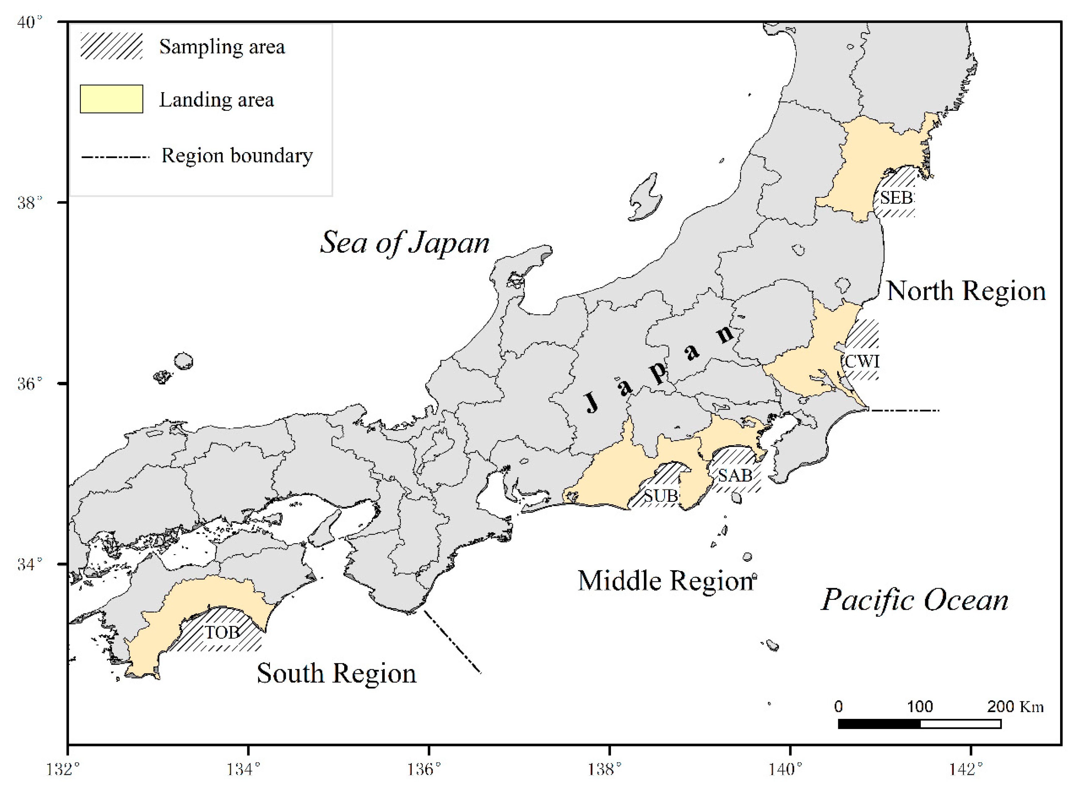
2.1. Sampling and Otolith Analysis

The anchovy larvae and juveniles used in this study were collected from bays or coastal waters off the Pacific coast of Japan’s five prefectures, across the Pacific North, Middle, and South fisheries regions (Ministry of Agriculture, Forestry and Fisheries of Japan; https://www.maff.go.jp/tokai/tokei/nenpo/68.html, accessed on 1 November 2022). Fish were obtained by commercial shirasu fishery, a local specialty fishery in Japan mainly for post-larvae and young juveniles of anchovy, sardine, and herring. Sampling (

Table 1. Summary of Japanese anchovy larvae and juvenile samples aged in this study.

Sampling Area	n	Range of Age (d)	Range of SL (mm)	Back-Calculated Spawning Season	Back-Calculated Spawning SST (°C)
SEB	92	23–67	18.11–32.91	May–September	12.2–27.1
CWI	228	22–50	17.82–33.80	April–October	12.7–25.8
SAB	146	21–44	18.13–32.49	February–July	15.7–23.4
SUB	293	23–54	16.21–39.38	February–May	15.8–18.2
TOB	599	17–64	12.96–36.29	January–May	16.9–20.8

, Figure 1) was conducted thrice a month during the spawning season in Sendai Bay (SEB), coastal waters off Ibaraki Prefecture (CWI), Sagami Bay (SAB), Suruga Bay (SUB), and Tosa Bay (TOB). Single-boat trawling was employed in SEB and SAB, while two-boat trawling was employed in the other three areas. The samples were immediately frozen at −20 °C (for fish in SEB, CWI, SAB, and SUB) or preserved in 70% ethanol (for fish in TOB). Measurements of standard length (SL, to the nearest 0.01 mm) and body weight (BW, in g to 4 decimal places) were conducted for each individual fish in the laboratory. We calculated the original size and weight of alcohol-preserved fish individuals from the shrinkage rate obtained from a subsample of 175 individuals (Figures S1 and S2). Sagittal otoliths were extracted under a dissecting microscope, washed in alcohol, and mounted on glass slides with clear nail polish.

The microstructure of otoliths (Figure S3) was captured at ×200 or ×400 magnification using a microscope (Leica DM2500, Germany) coupled with an optical camera system (Leica DFC295, Germany). The counting of increments was performed using ImageJ software (version 1.53e, United States National Institutes of Health; https://imagej.nih.gov/ij/, accessed on 5 October 2021) along the longest axis from primordia to edge, following the method named Group Band Reading [38]. The first distinctive increment at around 5–6 μm from the nuclei was determined to be formed at first feeding [39]. Incremental counts for each otolith were conducted three times with a two-month interval between each count. If the three counts for an otolith were different from each other, the counts would be rejected, and the otolith was excluded from subsequent analysis.

2.2. Aging and Environmental History Reconstruction

The daily periodicity of the increment deposition [40,41,42] has been validated for anchovy. Daily increments begin to be deposited on the sagittal otoliths of anchovy larvae at first feeding on day 4 after hatching [41]. Age was calculated as the number of increments plus three, and the date of hatching was back-calculated by subtracting the number of ages from the date of capture. The hatching of anchovy is thought to occur two days after spawning [21].

In this study, it was assumed that spawning of anchovy took place in the sampling areas and the larvae developed in these bays or coastal areas [43,44]. The environmental histories of the fish individuals were deduced from satellite monitoring data (published by CMEMS, https://marine.copernicus.eu/). Sea surface temperature (SST, °C) data were derived from OSTIA-UKMO L4 daily product with a spatial resolution of 4 km × 4 km, and chlorophyll-a concentration (Chl-a, mg·m⁻³) was obtained from ACRI-ST L4. The average daily SST and Chl-a values for each area were estimated (Figure 2).

2.3. Growth Analysis and Modeling

A total of 3166 frozen individuals from 59 sampling trips, ranging from 11 to 40 mm in body length, were used to estimate the parameters of the LWR. The relationship between body length and weight was described as

BW = aSL^b

(1)

Kn for each individual was calculated by using the following formula [33]:

$$K_n=\frac{W_o}{W_c}$$

(2)

where $W_o$ is the observed weight (g) of the fish specimens and $W_c$ is the calculated weight estimated from the LWR (Equation (1)).

In this study, the von Bertalanffy growth function and three sigmoidal (Gompertz, logistic, and Richards) functions were used to model the early growth of anchovy. The comparison and selection of candidate models were based on a multi-model inference (MMI) approach [45,46,47]. The model with the smallest AIC value and largest R-squared was considered to be the most representative of the growth pattern.

Logistic model:

$$L_t=L_{\infty }{\left(1+e^{-k\left(t-t_0\right)}\right)}^{-1}$$

(3)

von Bertalanffy model:

$$L_t=L_{\infty }\left(1-e^{-k\left(t-t_0\right)}\right)$$

(4)

Gompertz model:

$$L_t=L_{\infty }{e}^{-e^{-k\left(t-t_0\right)}}$$

(5)

Richards model:

$$L_t=L_{\infty }{[1+\left(d-1\right)e^{-k\left(t-t_0\right)}]}^{\frac{1}{1-d}}$$

(6)

where $L_t$ is the standard length in mm, $t$ the age in day, $k$ the growth-rate coefficient, and $L_{\infty }$ the asymptotic standard length. $t_0$ indicates the theoretical age of the fish when the standard length is 0 in the von Bertalanffy model and the age at the inflection point in the other three models. $d$ is a constant that in part determines the point of inflection on the $L_t$ axis. The inflection point is a point where the curvature of the graph changes from concave-upward to concave-downward and marks the highest growth rate.

SL at hatching was fixed at 2.9 mm [48], and thus the mean daily growth rate (${\mathrm{GR}}_m$) was calculated by subtracting 2.9 mm from body length and dividing by age.

$${\mathrm{GR}}_m=\frac{SL-2.9}{\mathrm{age}}$$

(7)

We utilized a set of mixed-effect models to explore the impact of endogenous and exogenous factors on the mean daily growth rate of larvae and juvenile anchovy. A detailed analysis was performed using the statistical program R 4.2.1 (R Core Team 2022), and the R-package lme4 was used to fit the models.

As most studies examined age-related growth rate variation, we used age as a primary consideration to detect differences in individual mean growth rates due to changes in growth rates with age. Age (at capture) and Kn were included in the models as fixed endogenous variables and laid the foundation for the model set framework. The response variable, mean daily growth rate (GR_m), and fixed effect variables were natural log-transformed and mean-centered to satisfy the model assumptions. These variables were mean centered to facilitate model convergence. We introduced the hatching date (HD) in the analysis as a random intercept effect variable, allowing for the mean growth rate of individuals hatched on the same day to be close to each other. The random Age slope for HD was also included in Equation (9) and compared with the random intercept-only model (Equation (8)), which allowed for the interpretation of birthday-varying growth rate–age relationships [49]. These two models were fitted using restricted maximum likelihood estimation (REML) and then compared using Akaike’s information criterion (AICc) to determine the best type of random effect structures.

Once the optimum type of random effect structure was determined, we investigated the fixed endogenous sources of growth variation. A set of models, including different combinations of fixed effects, were fitted using maximum likelihood (ML). Automated model comparison and selection were performed with R-package MuMIn, starting with the global model (Equation (10)) including Age, Kn, Area, SST, and Chl-a as fixed effect variables. All metric fixed effect variables were natural log-transformed and mean centered, where chlorophyll-a concentration values were first added by 1 and then taken as the natural logarithm. To quantify the difference in growth between areas, we included the term Area in the model. The categorical variable Area was introduced into the model as a fixed effect, which induced correlations among individuals within an area. Pairwise comparisons between areas were performed using the multiple comparison approach (R-package multcomp). Environmental variables (SST and Chl-a) were regarded as exogenous fixed effects, enabling us to investigate the impact of temperature and potential food supply on the growth rate. The optimal model was selected using AICc and then refitted using REML to obtain unbiased parameter estimates. Schooling behavior was obvious for anchovy post-larvae and juveniles [50]. To characterize the correlation between individuals within one school (caught on the same day), we introduced a random effect catch date (CD) replacing (HD) to demonstrate the heterogeneity in growth among different schools of fish. The CD-based model (Equation (11)) was fitted with REML, and the modeling performance was compared with that of the HD-based model.

$${\mathrm{GR}}_m={\alpha }_0+{\mathsf{\beta }}_1\mathrm{Age}+{\mathsf{\beta }}_2\mathrm{Kn}+{\mathsf{\beta }}_3\mathrm{Area}+{\alpha }_i+\epsilon$$

(8)

$${\mathrm{GR}}_m={\alpha }_0+{\mathsf{\beta }}_1\mathrm{Age}+{\mathsf{\beta }}_2\mathrm{Kn}+{\mathsf{\beta }}_3\mathrm{Area}+{\alpha }_i+b_i\mathrm{Age}+\epsilon$$

(9)

$${\mathrm{GR}}_m={\alpha }_0+{\mathsf{\beta }}_1\mathrm{Age}+{\mathsf{\beta }}_2\mathrm{Kn}+{\mathsf{\beta }}_3\mathrm{Area}+{\mathsf{\beta }}_4\mathrm{SST}+{\mathsf{\beta }}_5\mathrm{Chl}\_\mathrm{a}+{\alpha }_i+b_i\mathrm{Age}+\epsilon$$

(10)

$${\mathrm{GR}}_m={\alpha }_0+{\mathsf{\beta }}_1\mathrm{Age}+{\mathsf{\beta }}_2\mathrm{Kn}+{\mathsf{\beta }}_3\mathrm{Area}+{\mathsf{\beta }}_4\mathrm{SST}+{\mathsf{\beta }}_5\mathrm{Chl}\_\mathrm{a}+{\alpha }_j+b_j\mathrm{Age}+\epsilon$$

(11)

where ${\mathrm{GR}}_m$ is mean daily growth for fish individual and ${\alpha }_0$ represents overall averaged ${\mathrm{GR}}_m$ intercept. ${\mathsf{\beta }}_1$ (${\mathsf{\beta }}_2,$ ${\mathsf{\beta }}_3,$ ${\mathsf{\beta }}_4$, and ${\mathsf{\beta }}_5)$ represent fixed-effect Age (Kn, Area, SST, and Chl-a) coefficient. ${\alpha }_i$ is random effect for fish hatched in date $i$. $b_i$ is random Age slope for fish group hatched in date $i$, correlated with ${\alpha }_i$. ${\alpha }_j$ is random effect for fish caught in date $j$. $b_j$ is random Age slope for fish caught in date j, correlated with ${\alpha }_j$. $\epsilon$ represents error.

3. Results

3.1. Spawning Phenology

SST displayed analogous fluctuation among areas and years, going up gradually from April–May and then dropping from September. The SST in SEB is remarkably lower than that in other seas, especially in winter and spring. Overall, Chl-a concentration values were highest in spring, corresponding to the period when SST started to rise (Figure 2). A total of 1358 fish were aged from 17 to 67 days, with SL from 12.96 to 39.38 mm (Table 1). The estimated spawning dates ranged from January 20 to October 3 of 2020 and January 1 to August 11 of 2021, corresponding to spawning temperatures ranging from 12.2 to 27.1 °C or 18.5 °C on average (Table 1, Figure 2). The samples from SEB spawned over a wide range of temperatures, compared to the narrow spawning temperature range of those from SUB. In general, the spawning period in the south is earlier than that in the north. The spawning lasted from spring to autumn in CWI, and mainly occurred in late spring and summer in SEB. The spawning seasons in the other three areas were from late winter to spring (Figure 3). There was a large overlap between the spawning period and the period with high chlorophyll-a values (Figure 2 and Figure 3).

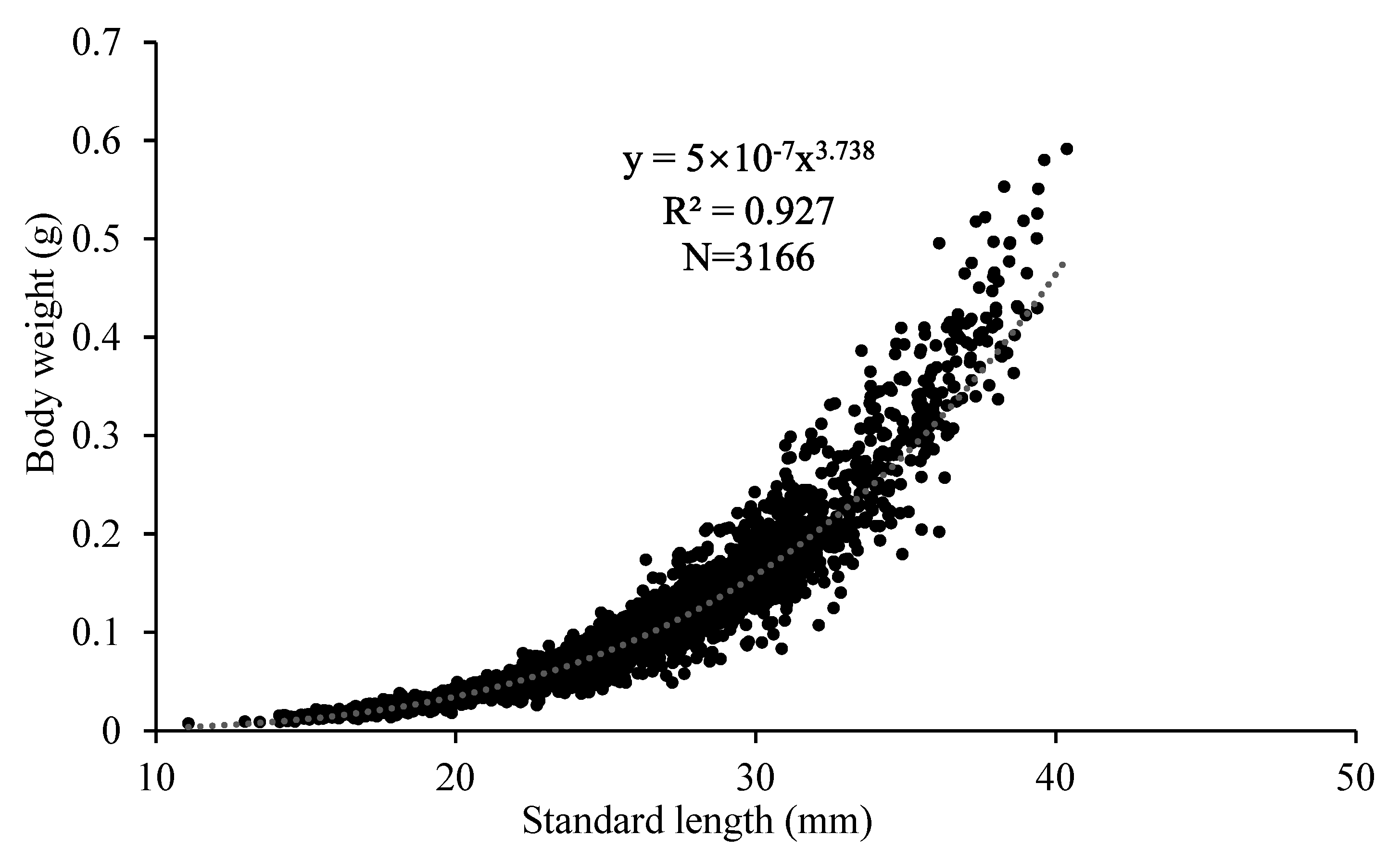
3.2. Length-Weight Relationship

The relationship equation for body length and weight was established as BW = 5 × 10⁻⁷SL^3.738 (Figure 4). The exponent b in the fitted equation for the LWR was significantly greater than 3 (Student’s t-test, p < 0.01), indicating strong positive allometric growth of anchovy during the study period.

3.3. Growth Function

The Gompertz model gave the best fit for the data set, with a growth rate parameter of 0.059 and an inflection point at the age of around 14 days (

Table 2. The parameter estimates and comparison of the growth models for larval and juvenile Japanese anchovy off the Pacific coast of Japan in 2020–2021.

Model	${\mathit{L}}_{\mathit{\infty }}$	$\mathit{k}$	$\mathit{d}$	${\mathit{t}}_0$	R2	AIC	∆AIC
Gompertz	34.23	0.059		14.26	0.6094	2569.19	0
Von Bertalanffy	35.87	0.042		5.22	0.6088	2569.29	0.10
Logistic	33.28	0.076		19.38	0.6086	2570.03	0.84
Richards	34.82	0.051	0.565	11.05	0.6086	2571.09	1.90

, Figure S4). The model revealed an acceleration in growth at the initial stage and a slowdown in growth after the age of inflection. The “best” models did not exhaustively account for the variation in length, with an explanation rate of about 60%. This demonstrates that fish of the same age varied in body length, and the mean growth rate varied among individuals.

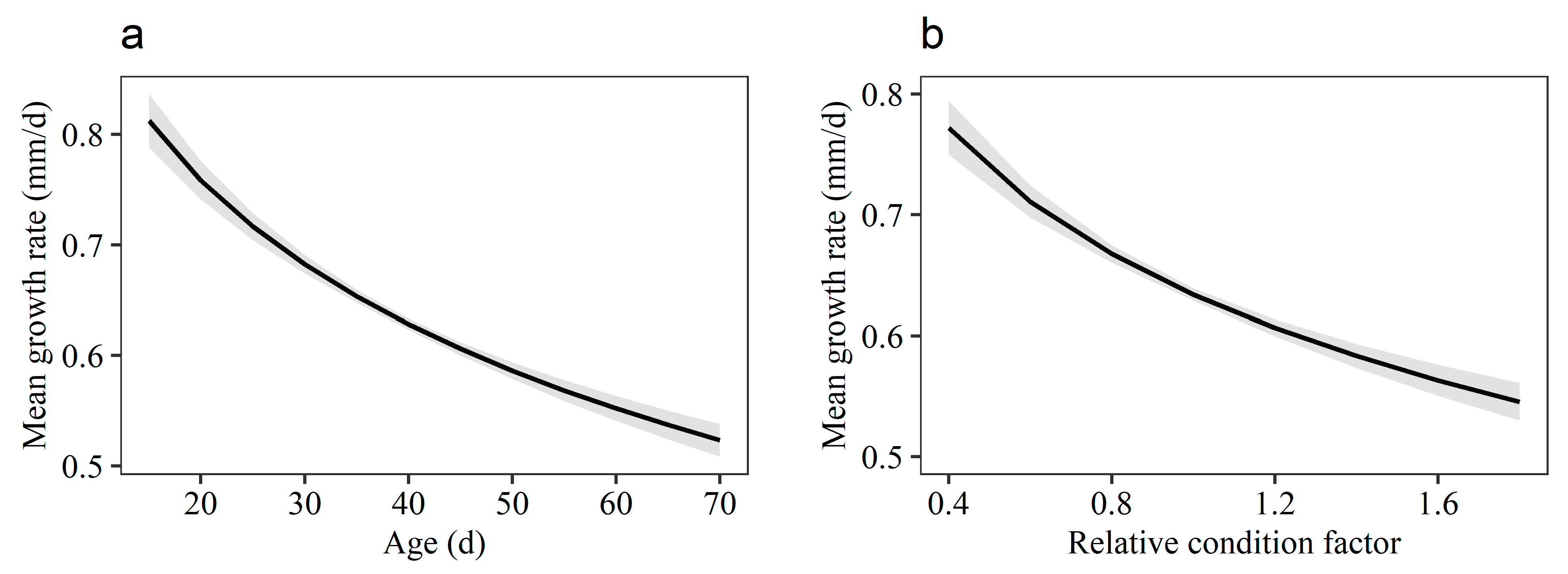
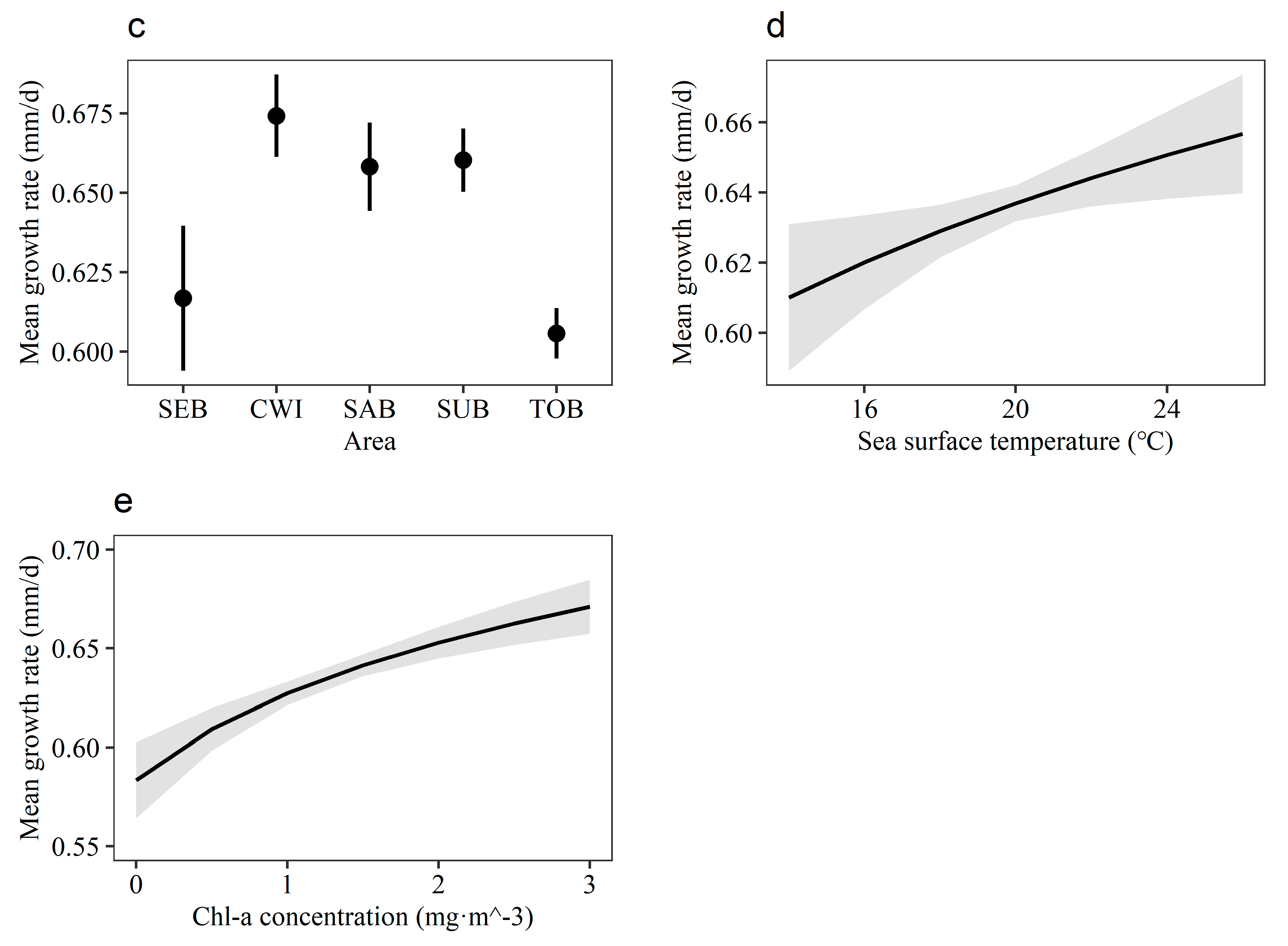
3.4. Growth Rate Variation among Individuals

Averaged over all individuals, the estimated mean daily growth rate for standard length was 0.64 ± 0.09 mm·day⁻¹. The model including the random Age slope and intercept for each HD performed better than the random intercept-only model, with a much smaller AICc value (Delta_AICc = 28.6). The random structure accounted for a correlation among individuals within a hatching date and presented differences in the mean growth of individuals born on different dates. The intraclass correlation coefficient (ICC) for HD was 0.30 (

Table 3. Parameter estimates (with CI and p) for the HD-based and CD-based model describing variation in mean daily growth rate of larval and juvenile Japanese anchovy off the Pacific coast of Japan in 2020–2021.

Predictors	HD-Based Model			CD-Based Model
	Estimates	CI	p	Estimates	CI	p
Intercept	−0.49	(−0.53, −0.46)	<0.001	−0.41	(−0.51, −0.32)	<0.001
Age	−0.29	(−0.33, −0.25)	<0.001	−0.32	(−0.40, −0.25)	<0.001
Kn	−0.24	(−0.28, −0.21)	<0.001	−0.21	(−0.25, −0.17)	<0.001
Area			<0.001			<0.001
SST	0.13	(0.04, 0.22)	0.004
Chl-a	0.10	(0.07, 0.14)	<0.001
Random effects	HD			CD
ICC	0.30			0.45
AICc	−2322.86			−2596.44
Marginal R2	0.444			0.429
Conditional R2	0.611			0.688

Notes: Empty cells mean that the parameter did not appear in the model. Marginal R² describes the proportion of variance explained by fixed effects alone, and conditional R² describes the proportion of variance explained by fixed and random effects combined.

), implying that the mean growth rates varied between individuals hatched on different dates, and that individuals with the same hatching date had approximate growth rates.

The global model containing all fixed effect variables was chosen as the optimal model, with the smallest AICc value and weighting dominantly among all possible models. The components that constitute the best endogenous effects were Age, Kn, and Area. As expected, the mean daily growth rate was generally negatively correlated with Age (Figure 5a, Table 3), indicating a decreasing trend in the daily growth rate during the studied age period. Meanwhile, there was a negative correlation between individual mean growth and Kn (Figure 5b, Table 3). An inherent difference was observed in the mean growth rate between the samples from the five areas. The optimal model predicted that the mean growth of fish varied across areas, with significantly higher growth for CWI, SAB, and SUB samples, and relatively lower growth for SEB and TOB samples (Figure 5c, Table S1). The optimal model showed that environmental factors SST and Chl-a were positively correlated with growth rate (Figure 5d,e, Table 3). The mixed-effects model explained more than 61% of the total variance of the data (conditional R²).

After changing the optimal model to include catch date instead of hatching date as a random effect, the new model had a significantly reduced AICc value and a significant improvement in the explanation rate (Table 3). The environmental variables SST and Chl-a were excluded from the CD-based model because of the non-significant effect on the response variable.

4. Discussion

The alternate population dynamics between anchovy and sardine in the western North Pacific were observed from long-term monitoring and catching data. However, Japanese anchovy stocks are relatively stable, as opposed to Japanese sardine stocks, which show 400-fold fluctuations from 1906 to 1984 [17]. One explanation is that the extraordinarily long spawning period and multiple spawning events of anchovy, accompanied by the ability to change its mode of life and spawning, act as a buffer against the impacts of environmental changes [17]. Oozeki et al. [51] reported that spawning activities of anchovy were observed over a wide temperature range, from 12 to over 30 °C. However, in recent years, the recruitment per egg (RPE) for anchovy has been very low, which is indicative of high early mortality [14].

Rearing experiments and field investigations revealed that the onset of spawning for anchovy is related to an increase above 15 °C in water temperature [18]. Temperature may be responsible for latitudinal and interannual fluctuations in spawning. Variations in anchovy spawning periods in the five areas reflect the timing difference of seawater warming at each location. Anchovy begins to appear in Sendai Bay in May and can be captured until November [52], during which sea surface temperatures are above approximately 15 °C (Figure 2 and Figure 3). The anchovy preferred the northeastern and southwestern parts of Sendai Bay [52], from which the samples for this study were collected. In the coastal waters off Ibaraki Prefecture, anchovy larvae and juveniles were also recorded to be caught in winter [14].

Area-specific spawning seems to be induced by temperature and food availability, as shown by the differences in anchovy spawning periods in various areas. Theoretically, anchovy may spawn throughout the year in TOB, SUB, and SAB, where the water temperature exceeds 15 °C at the coldest time of year (Figure 2.). However, we only caught samples from late winter to early summer. This may have been due to the high mortality of eggs and larvae caused by high sea water temperatures and low chlorophyll-a concentrations during the summer and autumn (Figure 2 and Figure 3). Predation is also a non-negligible source of mortality in early life stages, although the mortality was not examined in this study. Size-based predation is recognized as a factor that may regulate early life survival and levels of recruitment [3,53,54,55]. The catalyst of the end of spawning season is still an open question, unlike the start of spawning, which is attributed to the rise in water temperature. When comparing the spawning ecology of anchovy in two bays close in latitude, Osaka Bay and Wakasa Bay, it was found that the SST remained higher than 15 °C in autumn when females in Wakasa Bay stopped spawning [18]. Hayashi et al. [20] found that anchovy ended spawning with shortening of day length in the Pacific waters off northern Japan. As with population fluctuations, interannual fluctuations in spawning period and duration may occur in anchovy. From the perspective of Cushing’s hypothesis [2], anchovy spawning time and duration may fluctuate interannually, and the degree to which spawning matches temporally and spatially with favorable conditions is an important cause of interannual fluctuations in the population. A population regulation mechanism exists in the anchovy population that modifies reproductive patterns and regulates the number of individuals according to environmental conditions [17]. Fujita et al. [56] found temporal variations in the hatching period and early survival of anchovy in the central Seto Inland Sea in response to environmental factors that affect the replenishment process and lead to population fluctuations. During our study period, when the sea surface temperature rose smoothly in spring, the chlorophyll-a concentration peaked from March to July (Figure 2). This not only provided material and energy sources for consumption, weight increase, and gonad development to parents, but also provided eggs and larvae with suitable thermal conditions and abundant food. Moreover, the spawning dates in this study were back-calculated from otolith microstructure analyses and thus only applied to the survivors that were captured. Depending on the date of spawning or hatching, survival may be selective.

Positive allometric growth (b > 3 in LWR) in larval and juvenile anchovy has been reported in different sea areas [18,29,44], indicating that anchovy grows faster in weight than in length, or that the large specimens in the sample are in better condition than the small ones. However, the LWR of a specific species can vary according to sex, season, habitat, and life stage. Our estimation of exponent b was much higher than values 3.10 (geometric mean) in FishBase [57]. LWR may change during metamorphosis from larvae to juveniles. During the transition from fry to smolt, Chinook salmon (Oncorhynchus tshawytscha) becomes slenderer [58,59]. Le Cren [33] also found different growth stanzas for the perch (Perca fluviatilis). Most anchovy samples in this study were in the metamorphosing stage [10], during which the anchovy undergoes the most dramatic morphological and physiological changes throughout its lifetime. While previous studies have focused on examining the characteristics during metamorphosis in terms of length ratios of body parts and changes in body surface appearance, our study emphasizes that disproportionate growth in body length and weight may be another major feature during metamorphosis. Changes in LWR at different life history stages merit attention and can reveal the ecological aspects of life history.

Some growth models have proven more useful or suitable for certain species or families than others [60]. The von Bertalanffy model is commonly used to fit the size-at-age data for adult fish in fisheries science. A major limitation of the von Bertalanffy model is that it does not fit the first year of growth well, and the Gompertz model has been used to model the growth of young fish [60,61]. The Gompertz model is commonly used for clupeoid larvae and juveniles [62,63,64]. Growth was significantly explained by Gompertz models for Peruvian anchoveta (Engraulis ringens) larvae, pre-recruits, and recruits in northern Chile [62]. Hernandez and Castro [65] observed a slight decrease in growth rate with age of E. ringens larvae during the winter spawning season off central Chile and recommended that a nonlinear model (such as the Gompertz model) would better describe larval growth. In contrast to the logistic model, the Gompertz growth curve is asymmetric before and after the inflection point and has a shorter initial period of increasing growth [66].

The best-fit Gompertz model showed an inflection point at approximately 14 days of age, implying that growth increases until reaching the maximum growth rate at the inflection age. This result is consistent with previous reports of the growth pattern of this species [43], with maximum growth rates at 10–15 days of age and a gradual decline thereafter. However, the retracing of growth patterns can vary depending on the size range and model selection. The inflection point was at approximately 19 days of age according to the logistic model. Growth curves of the four growth models were very close to each other (Figure S4). The AIC values of the four growth models compared in this study were very similar, and none of them could fully explain the variation in body length (Table 2). The variability in body length of anchovy cohorts prompted us to further explore the sources of growth rate variation.

The difference in growth rates obtained from different ages is not easily attributable to environmental factors. Some studies have improved methods for distinguishing the inherent growth (which varies with age or body length) of fish from the influence of external factors. Shima et al. [67] eliminated age-dependent larval growth trends by fitting the growth models and obtaining residuals. Cordoleani et al. [68] used a specific growth rate rather than the absolute growth rate to remove the influence of body size on the growth of Chinook salmon (O. tshawytscha). A similar approach was applied in anchovy growth studies, and the growth rates were standardized to eliminate the effect of age in days [69]. Likewise, our study suggests that growth rate is age- or length-specific, and studies on the role of ambient factors directly on growth rate, without accounting for the variation in growth rates with age (inherent growth), can be prone to misperceptions.

The mean daily growth rate over all samples was 0.64 ± 0.09 (mean ± SD) mm·day⁻¹ in our study, which is consistent with previous studies conducted in Japanese coastal waters with the estimate of 0.6–0.7 mm·day^-1 [56,70,71]. The somatic growth rate decreased with increasing anchovy length in the Seto Inland Sea [37]. Growth rate for anchovy larvae and juveniles also decreased with age in I-lan Bay Taiwan and Sagami Bay Japan [43,44]. However, no obvious relationship between the mean growth rate and daily age was found in a study conducted in the offshore areas off Japan [69]. In the present study, the growth model explained that the source of variation in body length among individuals was partly due to differences in fish age, revealing a reduction in growth rate after approximately 2 weeks of age. The slowdown in growth after the inflection point age, indicated by the growth model, resulted in older individuals with longer relatively slow growth periods, which in turn led to a reduction in the mean growth rate. In other words, the decrease in the daily growth rate with age led to a lower mean growth rate in older fish. On the other hand, faster-growing fish individuals need to enhance their foraging activities to meet food consumption [72], or tend to be bolder and are more likely to encounter fishing gear [73]; thus, faster growing fish can easily be caught at a younger age.

From the results of LWR and growth models for larval and juvenile anchovy, it can be predicted that the growth rate of larval fish gradually increased in a short period after hatching and reached a maximum within two weeks, after which it gradually decreased and entered the metamorphosis period. During metamorphosis, the fish showed positive allometric growth as the body length growth rate decreased and the body weight growth rate increased. Such a growth pattern, as described above, may be an early developmental characteristic of an endogenous genetic nature at the stock level; however, the growth process can be influenced by endogenous and exogenous factors and exhibit individual-specific growth.

Variations in maternal or initial physical conditions, represented by different hatching dates, may be an endogenous source of individual growth differences. Yoneda et al. [13] revealed that variations in egg and larval traits (starvation tolerance and growth rate) of anchovy offspring are significantly affected by maternal prey availability. Differences in maternal conditions differentiate the early growth of offspring from different parents or batches [74]. The differences in egg and early larvae (such as diameter size and yolk sac nutrient storage) can also be carried over to subsequent life history stages [75].

In addition to age and maternally induced initial conditions, the endogenous factors affecting anchovy length growth explored in this study include the “trade-off” between length growth and weight growth. The cost of a higher body weight for the same length is that it takes longer time to reach that length. That is, faster length growth leads to a smaller relative body weight. This phenomenon appears to be similar to the “growth effect” on the otolith and somatic size relationship, where slower-growing larvae tended to have larger otoliths than faster-growing conspecifics at the same somatic size [26,76]. According to our findings, the body weight of slow-growing fish of a given size was larger than that of fast-growing fish. The size-specific growth rate of anchovy larvae in Hiuchi-nada, Seto Inland Sea, was found to decrease with body weight [37], which was explained by an increase with increasing weight in size-specific energy output rate related to the size-specific growth rate.

Growth characteristics have been used in stock identification and habitat suitability evaluation [77,78,79]. For the Pacific stock of anchovy off Japan (Figure 1), the Middle Region (Chiba-Mie prefecture) accounted for most of the catch, and the South Region (Wakayama-Miyazaki prefecture) had a smaller catch. After 1990, the catch in Boso-Joban waters (Chiba, Ibaraki, and Fukushima prefectures) fluctuated significantly. However, the proportion of the Tokai Sea (Mie-Kanagawa prefectures) has been increasing [14]. Differences in mortality-related growth rates may partially explain the regional differences in catches. As predicted by the growth rate model, early anchovy in the two southern and northern areas were expected to grow relatively slowly, while anchovy in the three middle areas grew rapidly.

In research on the impact of marine environmental factors on fish growth, van Denderen et al. [80] reported that average growth in pelagic fish is more significantly influenced by temperature than that in demersal and deep-living species. The relationship between early growth and temperature has been broadly described in different studies as having two relationships: (1) the daily growth rate increased with water temperature until approximately 27 °C, and (2) a dome-shaped curve with maximum growth at 22–23 °C [22]. Our study suggests that the growth of anchovy tends to accelerate with increasing temperature (Figure 5d). The SST data used in this study were satellite derived and may have overestimated the actual water temperatures at which they live. This is because anchovy larvae and juveniles have distinct diurnal vertical movement behavior and the ability to live at water depths of up to tens of meters [81].

The effect of food availability on growth cannot be easily measured. The density of copepods has been considered an indicator of food availability for larval and juvenile anchovy in field surveys [37,82,83,84]. The somatic growth rate for larval and juvenile anchovy was found to be dependent on food availability rather than temperature in Sagami Bay and Hiuchi-nada [37]. However, van Denderen et al. [80] discovered a positive effect of net primary production on average fish growth, and no correlation between fish growth and zooplankton production or biomass. Over large spatial scales, prey abundance estimates often fail to reflect the effective concentrations of prey available to fish larvae [85]. In the laboratory experiments, mixed diets resulted in higher growth rates than single prey diets for European anchovy (Engraulis encrasicolus) [86], which demonstrates the limitations of single-species abundances in reflecting food availability. The chlorophyll-a concentration is an indicator of phytoplankton abundance and biomass in coastal waters [87,88]. An increase in Chl-a (Figure 2) should be associated with an increase in food availability for anchovy, which do not directly consume phytoplankton. Copepods, the main food of anchovy, rely on phytoplankton as a staple to their diet. From the correspondence between the spawning period and the spring bloom, it is inferred that Chl-a can indirectly reflect prey abundance and availability for anchovy.

Food availability affects growth synergistically or mutually constraining with temperature. In relatively cool waters, anchovy growth rate is more strongly correlated with water temperature than with food availability, while in warmer waters, food availability is more closely correlated with water temperature in the Kuroshio–Oyashio transition zone [82]. However, temperature and chlorophyll-a concentrations are not the sole environmental factors that affect early growth. In this study, after the optimal mean growth rate model was changed by replacing the random effect hatching date with the catch date in our analysis, the environmental factors, SST and Chl-a, no longer exhibited significant effects on the mean growth rate (Table 3). This, combined with the large ICC value in the modified model (Table 3), suggests minor differences in mean growth rates for individuals from the same school, and that differences among fish school with different catch dates can be partially explained by the differences in mean Chl-a and SST among fish. Other ecological and physical factors, such as population density [89,90], intraspecific interactions [69], and dissolved oxygen [22,91], can affect the growth of vulnerable early stage fish. Schooling behavior can provide fish with foraging and anti-predator advantages. Prevalent schooling behaviors of anchovy post-larvae and juveniles have been recorded in both laboratory rearing and commercial fisheries [50]. Therefore, it is not surprising that fish with similar early environments within the same school exhibited significant homogeneity in growth. Waldron et al. [92] highlighted that growth rates should be compared between school groups to investigate the causes of variations in the average growth rate of juvenile Northern anchovy (Engraulis mordax).

5. Conclusions

In summary, this study presented the association between spawning period and environmental factors and demonstrated that the early growth of Japanese anchovy is influenced by both endogenous and exogenous factors. Fish growth is facilitated by an increase in temperature, as well as food abundance, as represented by the chlorophyll-a concentration. While much attention has been paid to the effects of marine environmental factors on the early development of anchovy, endogenous factors may also play an important role. Global analysis of fish growth rates [80] implies that global changes in fish growth are not only driven by physiological changes due to climate change but also by ecological dynamics and phylogenetic constraints. In our study, a decrease in the growth rate was observed in both the growth model and the average growth rate model as the fish aged. Length and weight are two aspects of fish growth, one of which may be prioritized at different life history stages. The trade-offs made by individual fish in terms of body length or weight growth may seem to make sense ecologically. Growth and survival during the early stages of teleost fish development are closely related. Further studies of reproduction and early growth should serve as a link to establish the relationship between fish population fluctuations and the marine environment.

References

1. Asch, R.G.; Stock, C.A.; Sarmiento, J.L. Climate change impacts on mismatches between phytoplankton blooms and fish spawning phenology. Glob. Chang. Biol. 2019, 25, 2544–2559. [Google Scholar] [CrossRef] [PubMed]
2. Cushing, D. Plankton Production and Year-class Strength in Fish Populations: An Update of the Match/Mismatch Hypothesis. In Advances in Marine Biology; Elsevier Applied Science Publishers Ltd.: London, UK, 1990; Volume 26, pp. 249–293. [Google Scholar] [CrossRef]
3. Houde, E.D. Emerging from Hjort's Shadow. J. Northwest Atl. Fish. Sci. 2008, 41, 53–70. [Google Scholar] [CrossRef]
4. Takasuka, A.; Sakai, A.; Aoki, I. Dynamics of growth-based survival mechanisms in Japanese anchovy (Engraulis japonicus) larvae. Can. J. Fish. Aquat. Sci. 2017, 74, 812–823. [Google Scholar] [CrossRef] [Green Version]
5. Morrongiello, J.R.; Walsh, C.T.; Gray, C.A.; Stocks, J.R.; Crook, D.A. Environmental change drives long-term recruitment and growth variation in an estuarine fish. Glob. Chang. Biol. 2014, 20, 1844–1860. [Google Scholar] [CrossRef]
6. Cowan, J.J.; Rose, K.; Devries, D. Is density-dependent growth in young-of-the-year fishes a question of critical weight? Rev. Fish Biol. Fish. 2000, 10, 61–89. [Google Scholar] [CrossRef]
7. Whitten, A.R.; Klaer, N.L.; Tuck, G.N.; Day, R.W. Accounting for cohort-specific variable growth in fisheries stock assessments: A case study from south-eastern Australia. Fish. Res. 2013, 142, 27–36. [Google Scholar] [CrossRef]
8. Lluch-Belda, D.; Crawford, R.J.M.; Kawasaki, T.; MacCall, A.D.; Parrish, R.H.; Schwartzlose, R.A.; Smith, P.E. World-wide fluctuations of sardine and anchovy stocks: The regime problem. South Afr. J. Mar. Sci. 1989, 8, 195–205. [Google Scholar] [CrossRef] [Green Version]
9. Schwartzlose, R.A.; Alheit, J.; Bakun, A.; Baumgartner, T.R.; Cloete, R.; Crawford, R.J.M.; Fletcher, W.J.; Green-Ruiz, Y.; Hagen, E.; Kawasaki, T.; et al. Worldwide large-scale fluctuations of sardine and anchovy populations. South Afr. J. Mar. Sci. 1999, 21, 289–347. [Google Scholar] [CrossRef]
10. Takahashi, M.; Watanabe, Y. Staging larval and early juvenile Japanese anchovy based on the degree of guanine deposition. J. Fish Biol. 2004, 64, 262–267. [Google Scholar] [CrossRef]
11. Li, H.; Zhang, X.; Zhang, Y.; Liu, Q.; Liu, F.; Li, D.; Zhang, H. Climate-Driven Synchrony in Anchovy Fluctuations: A Pacific-Wide Comparison. Fishes 2022, 7, 193. [Google Scholar] [CrossRef]
12. Boldt, J.L.; Thompson, M.; Rooper, C.N.; Hay, D.E.; Schweigert, J.F.; Quinn, T.J., II; Cleary, J.S.; Neville, C.M. Bottom-up and top-down control of small pelagic forage fish: Factors affecting age-0 herring in the Strait of Georgia, British Columbia. Mar. Ecol. Prog. Ser. 2019, 617, 53–66. [Google Scholar] [CrossRef] [Green Version]
13. Yoneda, M.; Fujita, T.; Yamamoto, M.; Tadokoro, K.; Okazaki, Y.; Nakamura, M.; Takahashi, M.; Kono, N.; Matsubara, T.; Abo, K.; et al. Bottom-up processes drive reproductive success of Japanese anchovy in an oligotrophic sea: A case study in the central Seto Inland Sea, Japan. Prog. Oceanogr. 2022, 206, 102860. [Google Scholar] [CrossRef]
14. Kinoshita, J.; Yasuda, T.; Watanabe, C.; Kamimura, Y. Stock assessment and evaluation for Japanese anchovy Pacific stock (fiscal year 2021). In Marine Fisheries Stock Assessment and Evaluation for Japanese Waters; Japan Fisheries Agency and Japan Fisheries Research and Education Agency: Tokyo, Japan, 2022; p. 50. Available online: https://abchan.fra.go.jp/digests2021/index.html (accessed on 17 October 2022). (In Japanese)
15. Tsuruta, Y. Internal regulation of reproduction in Japanese anchovy (Engraulis japonica) as related to population fluctuation. Can. Spec. Pub. Fish. Aquat. Sci. 1989, 108, 111–119. [Google Scholar]
16. Yatsu, A. Review of population dynamics and management of small pelagic fishes around the Japanese Archipelago. Fish. Sci. 2019, 85, 611–639. [Google Scholar] [CrossRef] [Green Version]
17. Funakoshi, S. Relationship between stock levels and the population structure of the Japanese anchovy. Mar. Behav. Physiol. 1992, 21, 1–84. [Google Scholar] [CrossRef]
18. Funamoto, T.; Aoki, I.; Wada, Y. Reproductive characteristics of Japanese anchovy, Engraulis japonicus, in two bays of Japan. Fish. Res. 2004, 70, 71–81. [Google Scholar] [CrossRef]
19. Takasuka, A.; Oozeki, Y.; Kubota, H.; Tsuruta, Y.; Funamoto, T. Temperature impacts on reproductive parameters for Japanese anchovy: Comparison between inshore and offshore waters. Fish. Res. 2005, 76, 475–482. [Google Scholar] [CrossRef]
20. Hayashi, A.; Goto, T.; Takahashi, M.; Watanabe, Y. How Japanese anchovy spawn in northern waters: Start with surface warming and end with day length shortening. Ichthyol. Res. 2019, 66, 79–87. [Google Scholar] [CrossRef]
21. Hayasi, S. A note on the biology and fishery of the Japanese anchovy Engraulis japonica (Houttuyn). Rep. Calif. Coop. Ocean. Fish. Investig. 1967, 11, 44–57. Available online: http://www.calcofi.com/publications/calcofireports/v11/Vol_11_Hayasi.pdf (accessed on 11 November 2022).
22. Yamamoto, K.; Saito, M.; Yamashita, Y. Relationships between the daily growth rate of Japanese anchovy Engraulis japonicus larvae and environmental factors in Osaka Bay, Seto Inland Sea, Japan. Fish. Sci. 2018, 84, 373–383. [Google Scholar] [CrossRef]
23. Takasuka, A.; Aoki, I. Environmental determinants of growth rates for larval Japanese anchovy Engraulis japonicus in different waters. Fish. Oceanogr. 2006, 15, 139–149. [Google Scholar] [CrossRef]
24. Tsujino, K. Daily growth of Japanese anchovy larvae Engraulis japonica in Osaka Bay. Bull. Osaka Prefect. Fish. Exp. Sta. 2001, 13, 11–18. (In Japanese) [Google Scholar]
25. Yasue, N.; Takasuka, A. Seasonal variability in growth of larval Japanese anchovy Engraulis japonicus driven by fluctuations in sea temperature in the Kii Channel, Japan. J. Fish Biol. 2009, 74, 2250–2268. [Google Scholar] [CrossRef] [PubMed]
26. Takasuka, A.; Oozeki, Y.; Aoki, I.; Kimura, R.; Kubota, H.; Sugisaki, H.; Akamine, T. Growth effect on the otolith and somatic size relationship in Japanese anchovy and sardine larvae. Fish. Sci. 2008, 74, 308–313. [Google Scholar] [CrossRef]
27. Tanner, S.E.; Vieira, A.R.; Vasconcelos, R.P.; Dores, S.; Azevedo, M.; Cabral, H.N.; Morrongiello, J.R. Regional climate, primary productivity and fish biomass drive growth variation and population resilience in a small pelagic fish. Ecol. Indic. 2019, 103, 530–541. [Google Scholar] [CrossRef]
28. Froese, R.; Thorson, J.T.; Reyes, R.B. A Bayesian approach for estimating length-weight relationships in fishes. J. Appl. Ichthyol. 2013, 30, 78–85. [Google Scholar] [CrossRef] [Green Version]
29. Zhu, W.-B.; Zhu, H.-C.; Wang, Y.-L.; Zhang, Y.-Z.; Lu, Z.-H.; Cui, G.-C. Heterogeneity of fork length-weight relationship for juvenile Engraulis japonicus based on linear mixed-effects models. J. Appl. Ecol. 2021, 32, 4532–4538. (In Chinese) [Google Scholar] [CrossRef]
30. Froese, R. Cube law, condition factor and weight-length relationships: History, meta-analysis and recommendations. J. Appl. Ichthyol. 2006, 22, 241–253. [Google Scholar] [CrossRef]
31. Koushlesh, S.K.; Sinha, A.; Kumari, K.; Borah, S.; Chanu, T.N.; Baitha, R.; Das, S.K.; Gogoi, P.; Sharma, S.K.; Ramteke, M.H.; et al. Length-weight relationship and relative condition factor of five indigenous fish species from Torsa River, West Bengal, India. J. Appl. Ichthyol. 2017, 34, 169–171. [Google Scholar] [CrossRef]
32. Jisr, N.; Younes, G.; Sukhn, C.; El-Dakdouki, M.H. Length-weight relationships and relative condition factor of fish inhabiting the marine area of the Eastern Mediterranean city, Tripoli-Lebanon. Egypt. J. Aquat. Res. 2018, 44, 299–305. [Google Scholar] [CrossRef]
33. Le Cren, E.D. The Length-Weight Relationship and Seasonal Cycle in Gonad Weight and Condition in the Perch (Perca fluviatilis). J. Anim. Ecol. 1951, 20, 201–219. [Google Scholar] [CrossRef] [Green Version]
34. Kodama, M.; Diamante, R.A.; Salayo, N.D.; Castel, R.J.G.; Sumbing, J.G. Growth Performance and Condition Factor of Juvenile Milkfish (Chanos chanos) Cultured in a Marine Pen in Relation to Body Size and Temperature. Jpn. Agric. Res. Quarterly: JARQ 2021, 55, 191–200. [Google Scholar] [CrossRef]
35. Allan, B.J.M.; Browman, H.I.; Shema, S.; Skiftesvik, A.-B.; Folkvord, A.; Durif, C.M.F.; Kjesbu, O.S. Increasing temperature and prey availability affect the growth and swimming kinematics of Atlantic herring (Clupea harengus) larvae. J. Plankton Res. 2022, 44, 401–413. [Google Scholar] [CrossRef] [PubMed]
36. Raab, K.; Llope, M.; Nagelkerke, L.A.; Rijnsdorp, A.D.; Teal, L.R.; Licandro, P.; Ruardij, P.; Dickey-Collas, M. Influence of temperature and food availability on juvenile European anchovy Engraulis encrasicolus at its northern boundary. Mar. Ecol. Prog. Ser. 2013, 488, 233–245. [Google Scholar] [CrossRef] [Green Version]
37. Zenitani, H.; Kono, N.; Tsukamoto, Y.; Masuda, R. Effects of temperature, food availability, and body size on daily growth rate of Japanese anchovy Engraulis japonicus larvae in Hiuchi-nada. Fish. Sci. 2009, 75, 1177–1188. [Google Scholar] [CrossRef]
38. Cermeño, P.; Uriarte, A.; Morales-Nin, B.; Cotano, U.; Álvarez, P. Setting up interpretation criteria for ageing juvenile european anchovy otoliths. Sci. Mar. 2008, 72, 733–742. [Google Scholar] [CrossRef] [Green Version]
39. Hwang, S.-D.; Song, M.-H.; Lee, T.-W.; McFarlane, G.A.; King, J.R. Growth of larval Pacific anchovy Engraulis japonicus in the Yellow Sea as indicated by otolith microstructure analysis. J. Fish Biol. 2006, 69, 1756–1769. [Google Scholar] [CrossRef]
40. Takahashi, M.; Watanabe, Y.; Kinoshita, T.; Watanabe, C. Growth of larval and early juvenile Japanese anchovy, Engraulis japonicus, in the Kuroshio-Oyashio transition region. Fish. Oceanogr. 2001, 10, 235–247. [Google Scholar] [CrossRef]
41. Tsuji, S.; Aoyama, T. Daily growth increments in otoliths of Japanese anchovy larvae Engraulis japonica. Nippon Suisan Gakkaishi 1984, 50, 1105–1108. [Google Scholar] [CrossRef] [Green Version]
42. Namiki, S.; Tanaka, H.; Katayama, S.; Funaki, O.; Aoki, I.; Oozeki, Y. Validation of daily increment formation in otoliths of immature and adult Japanese anchovy Engraulis japonicus. Fish. Sci. 2010, 76, 951–959. [Google Scholar] [CrossRef]
43. Takasuka, A.; Aoki, I.; Mitani, I. Three synergistic growth-related mechanisms in the short-term survival of larval Japanese anchovy Engraulis japonicus in Sagami Bay. Mar. Ecol. Prog. Ser. 2004, 270, 217–228. [Google Scholar] [CrossRef]
44. Chiu, T.; Chen, C. Growth and temporal variation of two Japanese anchovy cohorts during their recruitment to the East China Sea. Fish. Res. 2001, 53, 1–15. [Google Scholar] [CrossRef]
45. Katsanevakis, S. Modelling fish growth: Model selection, multi-model inference and model selection uncertainty. Fish. Res. 2006, 81, 229–235. [Google Scholar] [CrossRef]
46. Ong, J.J.L.; Rountrey, A.N.; Marriott, R.J.; Newman, S.J.; Meeuwig, J.J.; Meekan, M.G. Cross-continent comparisons reveal differing environmental drivers of growth of the coral reef fish, Lutjanus bohar. Coral Reefs 2016, 36, 195–206. [Google Scholar] [CrossRef]
47. Chang, S.-K.; Chou, Y.-T.; Hoyle, S.D. Length-Weight Relationships and Otolith-Based Growth Curves for Brushtooth Lizardfish off Taiwan With Observations of Region and Aging–Material Effects on Global Growth Estimates. Front. Mar. Sci. 2022, 9, 921594. [Google Scholar] [CrossRef]
48. Fukuhara, O.; Takao, K. Growth and larval behaviour of Engraulis japonica in captivity. J. Appl. Ichthyol. 1988, 4, 158–167. [Google Scholar] [CrossRef]
49. Doubleday, Z.A.; Izzo, C.; Haddy, J.A.; Lyle, J.M.; Ye, Q.; Gillanders, B.M. Long-term patterns in estuarine fish growth across two climatically divergent regions. Oecologia 2015, 179, 1079–1090. [Google Scholar] [CrossRef]
50. Masuda, R. Ontogeny of swimming speed, schooling behaviour and jellyfish avoidance by Japanese anchovy Engraulis japonicus. J. Fish Biol. 2011, 78, 1323–1335. [Google Scholar] [CrossRef] [Green Version]
51. Oozeki, Y.; Takasuka, A.; Kubota, H.; Barange, M. Characterizing spawning habitats of Japanese sardine, Sardinops melanostictus, Japanese anchovy, Engraulis japonicus, and Pacific round herring, Etrumeus teres, in the Northwestern Pacific. Calif. Coop. Ocean. Fish. Investig. Rep. 2007, 48, 191. [Google Scholar]
52. Okata, A. Ecological studies on the biological production of young amberfish community in the Sendai Bay. II. Relationships between food chains and fish fauna. Nippon Suisan Gakkaishi 1976, 42, 29–44. [Google Scholar] [CrossRef]
53. Bailey, K.; Houde, E. Predation on Eggs and Larvae of Marine Fishes and the Recruitment Problem. In Advances in Marine Biology; Blaxter, J.H.S., Southward, A.J., Eds.; Academic Press Inc.: New York, NY, USA, 1969; Volume 25, pp. 1–83. [Google Scholar] [CrossRef]
54. Takasuka, A.; Aoki, I.; Mitani, I. Evidence of growth-selective predation on larval Japanese anchovy Engraulis japonicus in Sagami Bay. Mar. Ecol. Prog. Ser. 2003, 252, 223–238. [Google Scholar] [CrossRef]
55. Takasuka, A.; Aoki, I.; Oozeki, Y. Predator-specific growth-selective predation on larval Japanese anchovy Engraulis japonicus. Mar. Ecol. Prog. Ser. 2007, 350, 99–107. [Google Scholar] [CrossRef]
56. Fujita, T.; Yamamoto, M.; Kono, N.; Tomiyama, T.; Sugimatsu, K.; Yoneda, M. Temporal variations in hatch date and early survival of Japanese anchovy ( Engraulis japonicus ) in response to environmental factors in the central Seto Inland Sea, Japan. Fish. Oceanogr. 2021, 30, 527–541. [Google Scholar] [CrossRef]
57. Froese, R.; Pauly, D. (Eds.) FishBase. World Wide Web Electronic Publication. Available online: https://www.fishbase.org (accessed on 22 August 2022).
58. Kimmerer, W.; Avent, S.R.; Bollens, S.M.; Feyrer, F.; Grimaldo, L.F.; Moyle, P.B.; Nobriga, M.; Visintainer, T. Variability in Length–Weight Relationships Used to Estimate Biomass of Estuarine Fish from Survey Data. Trans. Am. Fish. Soc. 2005, 134, 481–495. [Google Scholar] [CrossRef]
59. MacFarlane, R.B.; Norton, E.C. Physiological ecology of juvenile Chinook salmon (Oncorhynchus tshawytscha) at the southern end of their distribution, the San Francisco Estuary and Gulf of the Farallones, California. Fish. Bull. 2002, 100, 244–257. [Google Scholar]
60. Flinn, S.A.; Midway, S.R. Trends in Growth Modeling in Fisheries Science. Fishes 2021, 6, 1. [Google Scholar] [CrossRef]
61. Schnute, J. A Versatile Growth Model with Statistically Stable Parameters. Can. J. Fish. Aquat. Sci. 1981, 38, 1128–1140. [Google Scholar] [CrossRef]
62. Plaza, G.; Cerna, F.; Landaeta, M.F.; Hernández, A.; Contreras, J.E. Daily growth patterns and age-at-recruitment of the anchoveta Engraulis ringens as indicated by a multi-annual analysis of otolith microstructure across developmental stages. J. Fish Biol. 2018, 93, 370–381. [Google Scholar] [CrossRef]
63. Dulčić, J. Growth of anchovy, Engraulis encrasicolus (L.), larvae in the Northern Adriatic Sea. Fish. Res. 1997, 31, 189–195. [Google Scholar] [CrossRef]
64. Basilone, G.; Ferreri, R.; Mangano, S.; Pulizzi, M.; Gargano, A.; Barra, M.; Mazzola, S.; Fontana, I.; Giacalone, G.; Genovese, S.; et al. Effects of habitat conditions at hatching time on growth history of offspring European anchovy, Engraulis encrasicolus, in the Central Mediterranean Sea. Hydrobiologia 2018, 821, 99–111. [Google Scholar] [CrossRef]
65. Hernandez, E.H.; Castro, L.R. Larval growth of the anchoveta Engraulis ringens during the winter spawning season off central Chile. Fish. Bull. 2000, 98, 704. [Google Scholar]
66. Tabatabai, M.; Williams, D.K.; Bursac, Z. Hyperbolastic growth models: Theory and application. Theor. Biol. Med. Model. 2005, 2, 14. [Google Scholar] [CrossRef] [PubMed] [Green Version]
67. Shima, J.S.; Osenberg, C.W.; Noonburg, E.G.; Alonzo, S.H.; Swearer, S.E. Lunar rhythms in growth of larval fish. Proc. R. Soc. B: Biol. Sci. 2021, 288, 20202609. [Google Scholar] [CrossRef] [PubMed]
68. Cordoleani, F.; Holmes, E.; Bell-Tilcock, M.; Johnson, R.C.; Jeffres, C. Variability in foodscapes and fish growth across a habitat mosaic: Implications for management and ecosystem restoration. Ecol. Indic. 2022, 136, 108681. [Google Scholar] [CrossRef]
69. Nishikawa, H.; Itoh, S.; Yasuda, I.; Komatsu, K. Overlap between suitable nursery grounds for Japanese anchovy (Engraulis japonicus) and Japanese sardine (Sardinops melanostictus) larvae. Aquac. Fish Fish. 2022, 2, 179–188. [Google Scholar] [CrossRef]
70. Mitani, I. The biological studies on the larvae of Japanese anchovy, Engraulis japonica Houttuyn, in Sagami Bay. Kanagawa Pref. Fish. Exp. Sta. Rep. 1990, 5, 1–140. (In Japanese) [Google Scholar]
71. Aoki, I.; Miyashita, K. Dispersal of larvae and juveniles of Japanese anchovy Engraulis japonicus in the Kuroshio Extension and Kuroshio–Oyashio transition regions, Western North Pacific Ocean. Fish. Res. 2000, 49, 155–164. [Google Scholar] [CrossRef]
72. Werner, E.E.; Anholt, B.R. Ecological Consequences of the Trade-Off between Growth and Mortality Rates Mediated by Foraging Activity. Am. Nat. 1993, 142, 242–272. [Google Scholar] [CrossRef]
73. Biro, P.A.; Post, J.R. Rapid depletion of genotypes with fast growth and bold personality traits from harvested fish populations. Proc. Natl. Acad. Sci. USA 2008, 105, 2919–2922. [Google Scholar] [CrossRef] [Green Version]
74. Yoneda, M.; Kitano, H.; Tanaka, H.; Kawamura, K.; Selvaraj, S.; Ohshimo, S.; Matsuyama, M.; Shimizu, A. Temperature- and income resource availability-mediated variation in reproductive investment in a multiple-batch-spawning Japanese anchovy. Mar. Ecol. Prog. Ser. 2014, 516, 251–262. [Google Scholar] [CrossRef] [Green Version]
75. Wilson, S.M.; Buehrens, T.W.; Fisher, J.L.; Wilson, K.L.; Moore, J.W. Phenological mismatch, carryover effects, and marine survival in a wild steelhead trout Oncorhynchus mykiss population. Prog. Oceanogr. 2021, 193, 102533. [Google Scholar] [CrossRef]
76. Reznick, D.; Lindbeck, E.; Bryga, H. Slower Growth Results in Larger Otoliths: An Experimental Test with Guppies (Poecilia reticulata). Can. J. Fish. Aquat. Sci. 1989, 46, 108–112. [Google Scholar] [CrossRef]
77. Macdonald, P.; Angus, C.H.; Marshall, C.T. Spatial variation in life history characteristics of common megrim (Lepidorhombus whiffiagonis) on the Northern Shelf. J. Sea Res. 2013, 75, 62–68. [Google Scholar] [CrossRef]
78. Barrios, A.; Ernande, B.; Mahé, K.; Trenkel, V.; Rochet, M.-J. Utility of mixed effects models to inform the stock structure of whiting in the Northeast Atlantic Ocean. Fish. Res. 2017, 190, 132–139. [Google Scholar] [CrossRef] [Green Version]
79. McBride, R.S. The Continuing Role of Life History Parameters to Identify Stock Structure. In Stock Identification Methods, 2nd ed.; Cadrin, S.X., Kerr, L.A., Mariani, S., Eds.; Academic Press: San Diego, CA, USA, 2014; pp. 77–107. [Google Scholar] [CrossRef]
80. van Denderen, D.; Gislason, H.; van den Heuvel, J.; Andersen, K.H. Global analysis of fish growth rates shows weaker responses to temperature than metabolic predictions. Glob. Ecol. Biogeogr. 2020, 29, 2203–2213. [Google Scholar] [CrossRef]
81. Kuwahara, A. Diurnal changes in vertical distributions of anchovy eggs and larvae in the western Wakasa Bay. Nippon Suisan Gakkaishi 1984, 50, 1285–1292. [Google Scholar] [CrossRef]
82. Takahashi, M.; Watanabe, Y. Effects of temperature and food availability on growth rate during late larval stage of Japanese anchovy (Engraulis japonicus) in the Kuroshio-Oyashio transition region. Fish. Oceanogr. 2005, 14, 223–235. [Google Scholar] [CrossRef]
83. Zenitani, H.; Kono, N.; Tsukamoto, Y. Relationship between daily survival rates of larval Japanese anchovy (Engraulis japonicus) and concentrations of copepod nauplii in the Seto Inland Sea, Japan. Fish. Oceanogr. 2007, 16, 473–478. [Google Scholar] [CrossRef]
84. Yasue, N.; Doiuchi, R.; Yoshimoto, Y.; Takeuchi, T. Diet of late larval Japanese anchovy Engraulis japonicus in the Kii Channel, Japan. Fish. Sci. 2009, 76, 63. [Google Scholar] [CrossRef]
85. Houde, E.D. Mortality. In Fishery Science: The Unique Contributions of Early Life Stages; Fuiman, L.A., Werner, R.G., Eds.; Blackwell Publishing: Oxford, UK, 2002; pp. 64–87. [Google Scholar]
86. Garrido, S.; Saiz, E.; Peters, J.; Ré, P.; Alvarez, P.; Cotano, U.; Herrero, D.L.; de Murguía, A.M.; Irigoien, X. Effect of food type and concentration on growth and fatty acid composition of early larvae of the anchovy (Engraulis encrasicolus) reared under laboratory conditions. J. Exp. Mar. Biol. Ecol. 2012, 434–435, 16–24. [Google Scholar] [CrossRef] [Green Version]
87. Huot, Y.; Babin, M.; Bruyant, F.; Grob, C.; Twardowski, M.S.; Claustre, H. Does chlorophyll a provide the best index of phytoplankton biomass for primary productivity studies? Biogeosciences 2007, 4, 707–745. [Google Scholar] [CrossRef] [Green Version]
88. Wernand, M.R.; Van der Woerd, H.J.; Gieskes, W.W. Trends in Ocean Colour and Chlorophyll Concentration from 1889 to 2000, Worldwide. PLoS ONE 2013, 8, e63766. [Google Scholar] [CrossRef] [PubMed]
89. Cowan, J.H., Jr.; Rose, K.A.; Houde, E.D.; Wang, S.-B.; Young, J. Modeling effects of increased larval mortality on bay anchovy population dynamics in the mesohaline Chesapeake Bay: Evidence for compensatory reserve. Mar. Ecol. Prog. Ser. 1999, 185, 133–146. [Google Scholar] [CrossRef] [Green Version]
90. Boëns, A.; Grellier, P.; Lebigre, C.; Petitgas, P. Determinants of growth and selective mortality in anchovy and sardine in the Bay of Biscay. Fish. Res. 2021, 239, 105947. [Google Scholar] [CrossRef]
91. Ekau, W.; Auel, H.; Pörtner, H.-O.; Gilbert, D. Impacts of hypoxia on the structure and processes in pelagic communities (zooplankton, macro-invertebrates and fish). Biogeosciences 2010, 7, 1669–1699. [Google Scholar] [CrossRef] [Green Version]
92. Waldron, M.; Armstrong, M.J.; Prosch, R.M. Aspects of the variability in growth of juvenile anchovyEngraulis capensisin the southern Benguela system. South Afr. J. Mar. Sci. 1989, 8, 9–19. [Google Scholar] [CrossRef]
Figure 1. Sampling areas for Japanese anchovy larvae and juveniles.
Fishes 08 00011 g001
Figure 2. Daily sea surface temperature (upper) and five-day moving averaged chlorophyll-a concentration (lower) averaged over the broader sampling areas in 2020–2021.
Fishes 08 00011 g002
Figure 3. Spawning date distribution of anchovy samples in 2020–2021.
Fishes 08 00011 g003
Figure 4. Length–weight relationship of larval and juvenile Japanese anchovy off the Pacific coast of Japan in 2020–2021.
Fishes 08 00011 g004
Figure 5. Predicted variation in mean daily growth rate of larval and juvenile Japanese anchovy in 2020–2021, back-transformed to the original scale. (a) Age-dependent trends (mean with 95% CI). (b) Relationship between mean growth rate and relative condition factor. (c) Fishing-area-specific variation in mean daily growth rate. (d) Relationship between mean growth rate and sea surface temperature. (e) Relationship between mean growth rate and chlorophyll-a concentration.
Fishes 08 00011 g005aFishes 08 00011 g005b