Topological Charge of Propagation-Invariant Laser Beams


1
Image Processing Systems Institute of the RAS—Branch of FSRC “Crystallography & Photonics” of the RAS, 151 Molodogvardeyskaya St., 443001 Samara, Russia
2
Samara National Research University, 34 Moskovskoe Shosse, 443086 Samara, Russia
3
Lebedev Physical Institute, 221 Novo-Sadovaya St., 443034 Samara, Russia
*
Author to whom correspondence should be addressed.
Photonics 2023, 10(8), 915; https://doi.org/10.3390/photonics10080915
Submission received: 10 July 2023
/
Revised: 3 August 2023
/
Accepted: 6 August 2023
/
Published: 9 August 2023
(This article belongs to the Special Issue Advances and Application of Structured Light)
Abstract
:If a vortex propagation-invariant beam is given by all its intensity nulls, then its topological charge (TC) can be defined easily: its TC is equal to the sum of topological charges of all optical vortices in these intensity nulls. If, however, a propagation-invariant beam is given as a superposition of several light fields, then determining its TC is a complicated task. Here, we derive the topological charges of four different types of propagation-invariant beams, represented as axial superpositions of Hermite–Gaussian beams with different amplitudes and different phase delays. In particular, topological charges are obtained for such beam families as the Hermite–Laguerre–Gaussian (HLG) beams and two-parametric vortex Hermite beams. We show that the TC is a quantity resistant to changing certain beam parameters. For instance, when the parameters θ and α of the HLG beams are altered, the beam intensity also changes significantly, but the TC remains unchanged.
1. Introduction
Under propagation-invariant beams, we understand laser beams that conserve their intensity structure in the transverse section upon propagation in free space. An example of such beams is the Hermite–Laguerre–Gaussian (HLG) beams family. The HLG beams were first studied in [1] and found wide applications in modern optics. In [2], generalized HLG beams were obtained as well as their astigmatic transform. In [3], HLG beams were investigated in nonlinear medium. In [4], propagation of the HLG beams was studied in uniaxial crystals. In [5], propagation of the HLG beams was considered in a paraxial ABCD-system bounded by a square aperture. In [6], elegant HLG beams were obtained and the first three terms were given—nonparaxial corrections into the complex amplitude of such beams. In [7], a closed expression was given for incoherent HLG beams. In this work, the mutual intensity of the HLG beams was derived in the Shell model. In [8], the HLG beams were generated by using a metasurface. The HLG beams are a parametric beams family whose properties depend on the parameter. At a specific value of this parameter, the HLG beam reduces into the conventional Hermite–Gaussian (HG) beam. At another value of this parameter, the HLG beam reduces into the conventional Laguerre–Gaussian (LG) beam. It is known that the HG beams have zero topological charge (TC) and orbital angular momentum (OAM), whereas the LG beams have nonzero TC and OAM. However, it is still unknown which TC has the LG beam at an arbitrary value of the parameter.
The HLG beams are an example of propagation-invariant laser beams [9,10]. Propagation-invariant beams can be represented as an axial superposition of the HG beams (or LG beams) with different weight amplitudes and phase delays. Mathematically, the complex amplitude of propagation-invariant beams is equal to the sum of the HG beams with arbitrary complex coefficients. The sum of the indices of the Hermite polynomials in the HG beam should be constant. Then, all the HG beams in the superposition propagate with the same phase velocity and the transverse intensity distribution of the whole superposition change only in scale. The general expression for the OAM of a propagation-invariant superposition of the HG beams was derived in [11]. Propagation-invariant, including diffraction-free, beams found wide applications in optics [12,13]. They are used in fundamental physics [14], telecommunications [15,16,17], optical cryptography [18,19,20], micromachines [21,22], imaging systems [23,24,25,26], and for manipulating biological objects (cells) [27,28]. Interesting studies were conducted in the works [29,30,31], studying the propagation-invariant beams, which are different from the HLG beams since each coefficient in the superposition of the HG beams was multiplied by a respective power of a complex number. At a certain value of this complex number, the OAM of such beams becomes zero, while at a small change of this complex number, the OAM changes abruptly. In the works [29,30,31], the expressions for the OAM were derived, but the TC of such generalized HLG beams was not considered in these works.
Obtaining the TC of propagation-invariant beams represented as a superposition of the HG beams with uncertain complex weights is generally a problem, equivalent by complexity to finding all zeros of a certain polynomial, given by its coefficients. The TC of such a superposition can be found for certain parametric laser beam families. In this work, we analytically derive the TC of the parametric family of the HLG beams at an arbitrary value of the parameter. In addition, we obtain the TC of several other propagation-invariant beams, for instance, two-parametric vortex Hermite–Gaussian beam, which is different from the single-parametric beam [32].
For convenience, we define here several terms important for this work. Vortices are screw wavefront dislocations of a laser beam. They are also called phase singularities. In the center of each vortex, the phase is undetermined and the intensity is therefore zero in these points. Thus, the vortices in the beam section can be detected by isolated intensity nulls. The topological charge of an optical vortex is an integer number of phase jumps by 2π along a closed contour of a large radius in the laser beam section. Thus, to obtain the TC, the phase distribution of the beam should be known. Orbital angular momentum density in each point of the beam section is defined as a product of conjugated complex amplitude E*(r, φ) and of its azimuthal angle derivative dE(r, φ)/dφ, where (r, φ) are the polar coordinates in the beam section. Physically, a nonzero OAM of a light beam means that the energy flow in the beam is propagating along a spiral.
2. Propagation-Invariant Vortex Fields with Multiple Phase Singularities
As was shown in [9,10], an arbitrary function given by
where (x, y, z) are the Cartesian coordinates, w is the waist radius of the Gaussian beam, q = 1 + iz/z0, is the Rayleigh distance, λ is the wavelength, and f (x ± iy) is an arbitrary integer analytical function, is a solution to the paraxial Helmholtz equation:
Formula (1) describes propagation-invariant light fields with their intensity distribution conserving upon propagation in space (up to a scale and rotation around the optical axis). The rotation direction (clockwise or counter-clockwise) is defined by choosing the sign in the argument of the function f. Below, without loss of generality, we consider light fields with the sign “+”. Formula (1) allows for an analytical description of light fields with arbitrary locations of optical vortices [9,10] in arbitrary plane z in the points with the Cartesian coordinates (ak, bk) (k = 1,..., M):
The topological charge (TC) of a light field can be obtained by the M.V. Berry’s formula [33]:
applied to the complex amplitude in the polar coordinates x = r cos φ, y = r sin φ.
Formula (4) makes it possible to obtain the TC of an even more general beam, that instead of the Gaussian function in Equation (3) is described by an arbitrary (even complex) radially symmetric multiplier A(r). If the isolated intensity nulls of a propagation-invariant beam in the initial plane reside in point with the coordinates , then the complex amplitude of such a beam is given by
where mk are integer numbers equal to multiplicities of the intensity nulls.
Substituting Equation (5) into Equation (4), we obtain
Thus, the TC of a propagation-invariant beam with M intensity nulls, each with a multiplicity mk, is equal to the sum of these multiplicities. If the beam has optical vortices with both positive TCs and negative TCs, then its complex amplitude reads as
Similarly to Equation (6), the TC of the beam (7) can be obtained as
The result (8) is almost obvious, since it means that the TC of a beam with M positive intensity nulls and with N negative nulls is equal to the algebraic sum of multiplicities of all the nulls in the beam section. We note that the beam (7) is no longer propagation-invariant.
3. Topological Charge of the Hermite–Laguerre–Gaussian Beams
In practice, the positions of the intensity nulls and their multiplicity are not known, and in the experiment they can be found only by generating a interference pattern with forks. Instead of explicitly defining a light field by its intensity nulls (3) or (5), a light field can be represented by polynomials or their linear combinations. Since the Hermite–Gaussian (HG) beams and the Laguerre–Gaussian (LG) beams are propagation-invariant beams themselves, then a large amount of propagation-invariant beams can be represented as a finite superposition of HG or LG beams, for instance, by HG beams with their indices yielding the constant Gouy phase. Thus, below we study paraxial beams with complex amplitude being equal to a finite sum of the HG beams with the indices, the sum of which is a constant:
Here, ck are arbitrary complex coefficients and Hk(x) are the Hermite polynomials defined by the following recurrent relation:
with the first two polynomials equal to , .
Mathematically, the propagation invariance of the HG beams upon propagation can be expressed by via the Fresnel transform:
where , z0 = πw2/λ is the Rayleigh distance, λ is the wavelength of light, (ξ, η) and (x, y) are the transverse Cartesian coordinates in the initial plane and at a distance z, z is the third Cartesian coordinate directed along the optical axis of the beam, and is the Gouy phase. As seen from Equation (11), the HG beams with a constant sum of indices, i.e., with n + m = N, propagate with the same phase velocity, and therefore a superposition (9) of such beams is propagation-invariant. Below, we use dimensionless coordinates x = x/w, y = y/w for brevity.
In a general case, if the complex coefficients ck are arbitrary, the TC of the field (9) cannot be found. Below, we obtain the TC for two families of propagation-invariant fields: for vortex Hermite beams and for Hermite–Laguerre–Gaussian (HLG) beams.
We start from the latter ones. The complex amplitude of the HLG beams in the initial plane can be represented as a superposition of the HG beams [1]:
The vertical line in the left part is a separator between the arguments (x, y) and the parameter θ, coefficients are pure real trigonometric polynomials of θ and are expressed via the Jacobi polynomials:
The orbital angular momentum (OAM) of the beams (12) is known [1] and equals , but the TC was not yet derived theoretically. It is seen that if θ = 0 then, since sin 0 = 0, only one term with k = m remains in the expansion (12). In this case, and the HLG beam reduces into an HG beam:
The topological charge of the HG beams is zero. It is easy to note that the HLG beam reduces into the HG beam also at other values of the parameter θ: π/2, π, 3π/2, 2π, since in these cases also only one term remains in the sum (12). Thus, for these values of the parameter θ, the TC of the beam (12) is also equal to zero. However, at θ = π/4, the HLG beam reduces into an LG beam:
with being the associated Laguerre polynomial. Evidently, the TC of the HLG beam in this case is equal to . Thus, a question arises: if the TC of the beam (12) is equal to zero at θ = 0, π/2, and is equal to at θ = π/4, then what is the TC value at other values θ from the interval (0, π/2)? For obtaining the TC of the HLG beams in the general case, we use an interesting property of the coefficients [1]:
According to Equation (4), the TC of a light field is obtained in the limit of arguments x and y tending to infinity. Using an asymptotic expression of the Hermite polynomials, , we obtain for the beam (12):
It is seen from Equation (17) that two elliptic optical vortices with the topological charges n and –m interact in the origin (x = y = 0). Thus, according to Equation (8), the TC of the whole field equals . Therefore, the TC of the beam (12) is equal to at an arbitrary value θ from the interval (0, π/2). The right part of the Formula (17) reveals that if θ is equal to π/2, π, 3π/2, or 2π, then the optical vortices disappear. In addition, if m = n and θ = π/4, the central optical vortex in the origin is also absent:
From Equation (17) follows that, in the second quarter of the angle θ variation period, i.e., in the interval (π/2, π), there are optical vortices with the topological charges –n and m in the origin. Thus, the TC of the beam (12) is equal to , i.e., changing the parameter θ makes it possible to change the TC sign of the HLG beam. It is interesting to compare the OAM of the HLG beam, , and its TC, . It is seen that the TC is independent of the parameter θ while it is, for instance, in the interval (0, π/4), whereas the OAM for different θ changes from zero to maximum. We note that multiplying all the coefficients (12) by a respective power of a real-valued parameter α, , can only change the sign of the TC of the HLG beam, since in this case we obtain instead of Equation (18):
4. Topological Charge of a Two-Parametric Vortex Hermite Beam
Propagation-invariant vortex Hermite beams were introduced and investigated in [33]. They are yet another example of the beam (9), whose coefficients allow the sum (9) to be written in a closed form and thus the TC can be obtained. To do this, we use the summation formula of the Hermite polynomials [34]:
Then, for applying the summation Formula (19) for simplifying the sum (9), the coefficients in Equation (9) should be chosen as follows:
Thus, the beam (9) with the coefficients (20) reads as
According to Equation (21), if the beam parameters t and τ are real and not equal to each other, then all zeros of the Hermite polynomial, each being real-valued and residing on the horizontal axis y = 0, generate elliptic optical vortices (screw dislocations) with a unit TC if tτ > 0 and with the TC of −1 if tτ < 0. The topological charge of the whole beam (21) is equal to the number of roots, i.e., n + m if tτ > 0 and –(n + m) if tτ < 0. Thus, in the second case of Equation (21), the TC of a propagation-invariant beam (9) is greater by magnitude than the TC of the beam (12). If t = τ, the vortex Hermite beam (21) reduces to a single-ringed Laguerre–Gaussian beam and all elliptic optical vortices merge into a single standard circular optical vortex in the origin, whose topological charge is still equal either to n + m or to –(n + m). It is interesting that the TC of the beam (21) is not changed with changing parameters if these parameters t and τ do not change their sign.
5. Simple Optical Vortices
If we substitute the following binomial coefficients
into Equation (9), then we derive an asymptotic expression for large values of the arguments, similar to the sum (17):
As seen from Equation (23), the asymptotic argument is equal to (n + m)φ, where φ is the polar angle in the beam cross-section. Therefore, the TC of the field (9) with the coefficients (22) equals n + m. For deriving Equation (23), the Newton’s binomial theorem [34] was used:
Another example of determining the topological charge of a superposition of optical vortices can be given by using the following finite sum [35]:
where P2n(x) are the Legendre polynomials, orthogonal in the interval [−1, 1], and having n simple real-valued zeros in this interval. Then, the asymptotic expression for large argument values for the beam (9) is given by
For deriving Equation (26), the summation coefficients in Equation (9) were chosen as follows:
According to Equation (26), the TC of the beam (9) with the coefficients (27) is equal to n + m, since there is an elliptic optical vortex in the center of the beam section, whose amplitude is proportional to an expression . The Legendre polynomial does not have additional zeros since the real value of the Legendre polynomial argument in Equation (26) equals 1. We note that if the coefficients (22) and (27) are multiplied by a real-valued parameter α, i.e., , then such change in the coefficients changes the intensity distribution of the propagation-invariant beam (9) and changes its OAM, but does not change its TC.
6. Propagation-Invariant Beams in the Laguerre-Gaussian Basis
Instead of the HG basis, the complex amplitude of propagation-invariant light fields can be written in the Laguerre–Gaussian (LG) basis:
In Equation (28), there are Laguerre polynomials in the sum, (r, φ) are the polar coordinates in the waist plane of the LG beam. The square brackets in Equation (28) denote the integer part of a number. Below, we use a dimensionless radial variable r instead of the ratio r/w and limit our study by considering only positive-charge optical vortices, i.e., we choose the plus sign in Equation (28). The topological charge of the optical vortices superposition (28) can be determined by obtaining the argument (phase) of an asymptotic expression (28) when x and y tend to infinity. For this purpose, we apply an asymptotic expression for the Laguerre polynomials (r >> 1):
Then, instead of Equation (28), we write an asymptotic expression for the amplitude of beams (28):
It is difficult to obtain the TC of the superposition (30) for arbitrary real coefficients ck. Therefore, we consider only several partial cases that allow for a closed-form representation of the sum in Equation (30). We note that at certain coefficients values, the superposition of optical vortices (30) reduces to the geometrical sequence. The TC in the geometrical sequence of optical vortices was obtained in [36]. Therefore, we consider other examples of choosing the coefficients in Equation (28). We use the well-known sum following from Newton’s binomial theorem [35]:
Then, choosing in Equation (30) the following coefficients:
we obtain instead of Equation (30) the following expression:
As seen from Equation (33), the argument of the asymptotic expression is equal to (Nφ)/2, and the TC of the superposition (28) with the coefficients (32) is thus equal to N/2. As was shown in [36], the half-integer TC in the initial plane becomes integer and equal to N upon propagation of the beam (28). Similarly, other examples of the sums (31) can be considered, many of which were given in [35].
7. Numerical Simulation
A numerical simulation of the propagation of all the beams in this work was conducted by the Fresnel transform implemented as the convolution by using the fast Fourier transform. The obtained distributions we compared with the respective theoretical formulae for the complex amplitudes. Numerical and theoretical intensity distributions were visually indistinguishable, whereas the phase distributions were different only in the areas of negligible low intensity. The topological charge of all the considered beams was computed as a sum of the phase (argument of the complex amplitude) derivatives by the azimuthal angle, computed over a circle of a "large" radius with small light intensity, and divided by the full angle of 2π. As seen in all the figures below, the beams are propagation-invariant, i.e., conserve their intensity structure and change only in scale.
7.1. Simulation of the Hermite–Laguerre–Gaussian Beams
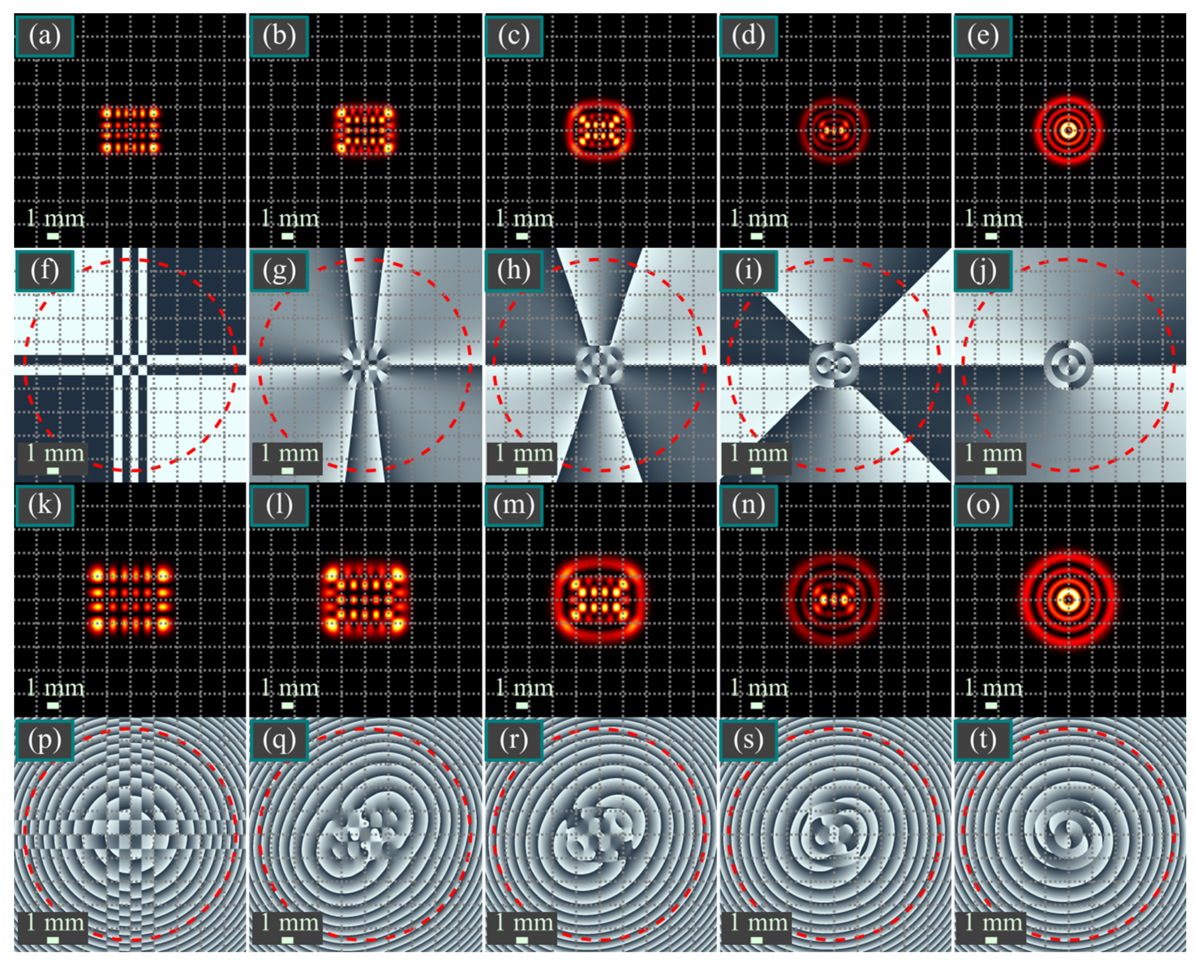
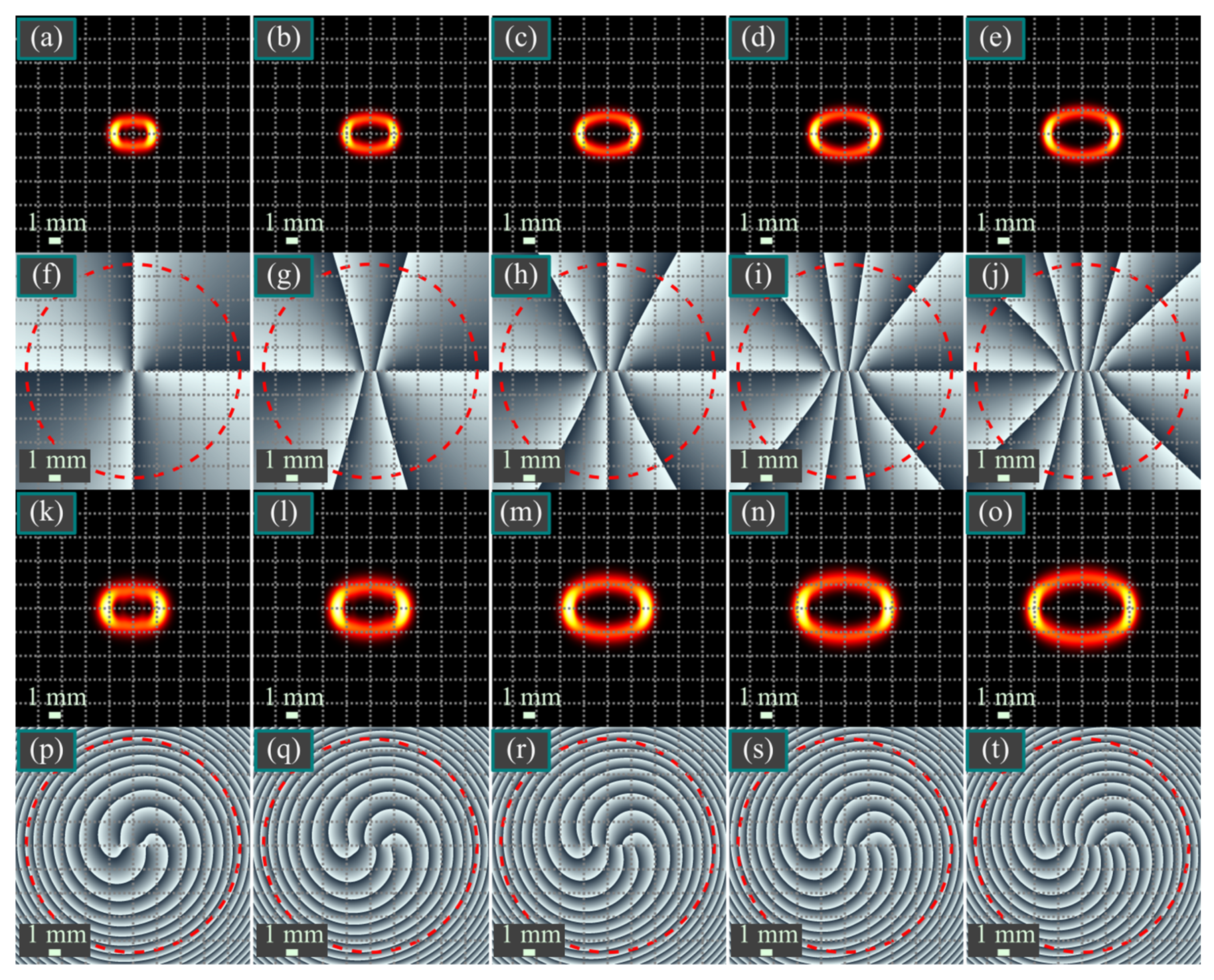
Figure 1 illustrates the intensity and phase distributions of the HLG beams (12) at (n, m) = (5, 3) for different values of the parameter θ: 0, π/16, π/8, 3π/16, π/4 in the initial plane z = 0 and at the Rayleigh distance z = z0. Shown in Figure 2 are also the intensity and phase distributions of the HLG beams (12) for the same values of the parameter θ and for the same propagation distances z, but at (n, m) = (2, 7). Both these figures confirm that, when θ changes from 0 till π/4, the HG beam with (n + 1) × (m + 1) light spots is converted into an LG beam with min(n, m) + 1 light rings. Computation of the topological charge over the phase distributions from Figure 1 yielded the following values: 0.000000 (Figure 1f), 1.999466 (Figure 1g), 1.999875 (Figure 1h), 1.999973 (Figure 1i), 1.999995 (Figure 1j), 0.000001 (Figure 1p), 1.994684 (Figure 1q), 1.993242 (Figure 1r), 1.992495 (Figure 1s), 1.992265 (Figure 1t). Thus, computation confirms that the TC is zero at θ = 0 and the TC is equal to 2 (n − m = 5 − 3 = 2) for all other values of θ. Phase distributions in the initial plane, shown in Figure 1, clearly indicate the TC values. On the dashed red circle in Figure 1f, there are only phase jumps by +π (when black color is changed to white, counter-clockwise) and by –π (when white color is changed to black). In total, all these jumps yield zero. Thus, the TC of a beam from Figure 1a,f is zero. As is clearly seen in Figure 1g–i, there are four nonhorizontal rays, where the phase on the dashed circle is changed by +2π, and two horizontal rays, where the phase on the circle jumps by –2π. Thus, the TC of the beams from Figure 1g–i equals 4 − 2 = 2. Finally, in Figure 1j, the dashed circle is intersected by two horizontal rays, where the phase is changed by 2π. Thus, the TC of the beam from Figure 1j is equal to 2. The same way, the TC can be simply computed for all other figures in this work.
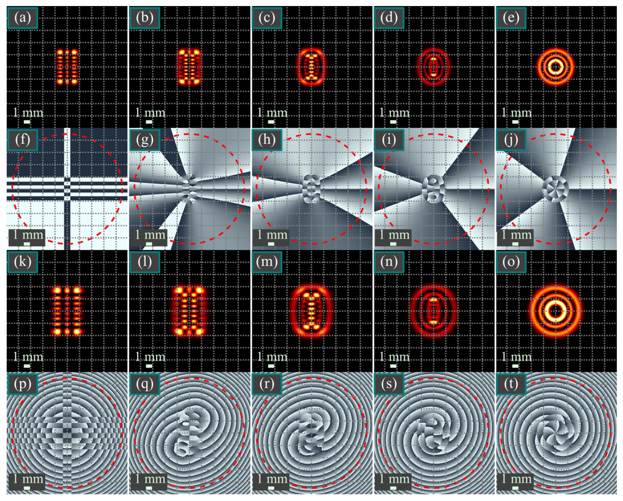
For Figure 2, the computed TC values are 0.000000 (Figure 2f), –4.998308 (Figure 2g), –4.999542 (Figure 2h), –4.999854 (Figure 2i), –4.999926 (Figure 2j), –0.000001 (Figure 2p), –4.986253 (Figure 2q), –4.982896 (Figure 2r), –4.981142 (Figure 2s), and –4.980602 (Figure 2t). This confirms that the TC is zero at θ = 0 and the TC is –5 (n − m = 2 − 7 = −5) for all other θ values.
Combining the TC computation results found in Figure 1 and Figure 2, we obtain that the TC of the beam from Equation (12) is equal to n − m for an arbitrary value θ from the interval (0, π/2), which is consistent with the above theory.
Figure 3 depicts the intensity and phase distributions of an HLG beam (12) from Figure 1c,h,m,r (n = 5, m = 3, θ = π/8) for different values of the parameter α (1, 0.8, 0.6, 0.4, 0.2) in the initial plane z = 0 and at the Rayleigh distance z = z0. According to Figure 3, with a decreasing value of the parameter α, the HLG beam of the order (n, m) reduces into a Hermite beam of the order (n + m, 0). Computation of the topological charge over the phase distributions from Figure 3 yielded the following values: 1.999871 (Figure 3f), 1.999796 (Figure 3g), 1.999654 (Figure 3h), 1.999347 (Figure 3i), 1.998661 (Figure 3j), 1.993265 (Figure 3p), 1.995472 (Figure 3q), 1.998142 (Figure 3r), 2.001121 (Figure 3s), and 2.003653 (Figure 3t). Thus, the computation confirms that the TC is equal to n − m = 5 − 3 = 2 at arbitrary values of α.
7.2. Simulation of Two-Parametric Vortex Hermite Beams
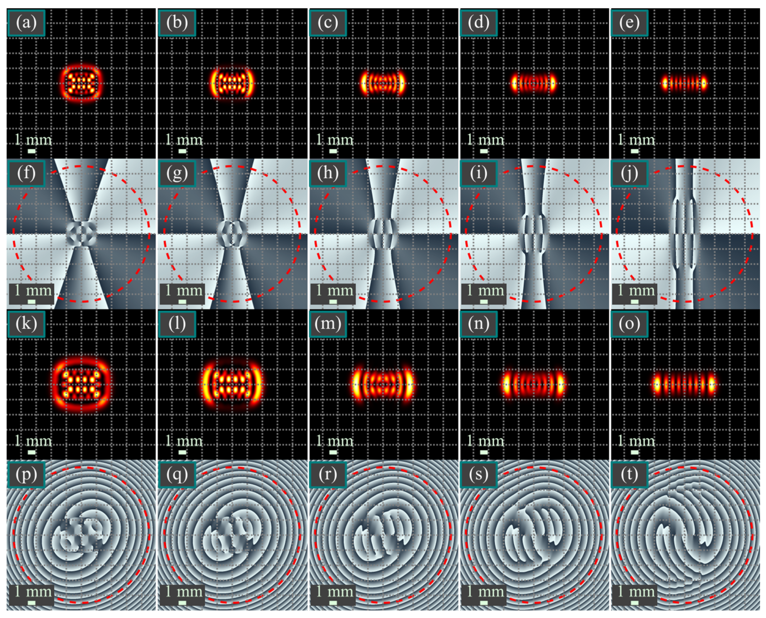
Shown in Figure 4 are the intensity and phase distributions of a two-parametric vortex Hermite beam (21) at (n, m) = (2, 7) for different values t and τ ((0.7, 0.7), (0.7, 0.4), (0.7, –0.3), (0.7, 0.2), (0.7, –0.1)) in the initial plane z = 0 and at the Rayleigh distance z = z0. According to Equation (21), when the magnitude of the parameter τ decreases, the beam should tend to the Hermite–Gaussian beam of the order (n + m, 0). Figure 4 confirms this. Computation of the topological charge over the phase distributions from Figure 4 yielded the following values: 8.999570 (Figure 4f), 8.999303 (Figure 4g), –8.998908 (Figure 4h), 8.997925 (Figure 4i), –8.994937 (Figure 4j), 8.964787 (Figure 4p), 8.966616 (Figure 4q), –8.968667 (Figure 4r), 8.972072 (Figure 4s), and –8.977350 (Figure 4t). Thus, computation confirms that the TC is equal to n + m = 2 + 7 = 9 if tτ > 0 and –(n + m) = –(2 + 7) = −9 if tτ < 0.
7.3. Simulation of Propagation-Invariant Beams in the Laguerre–Gaussian Basis
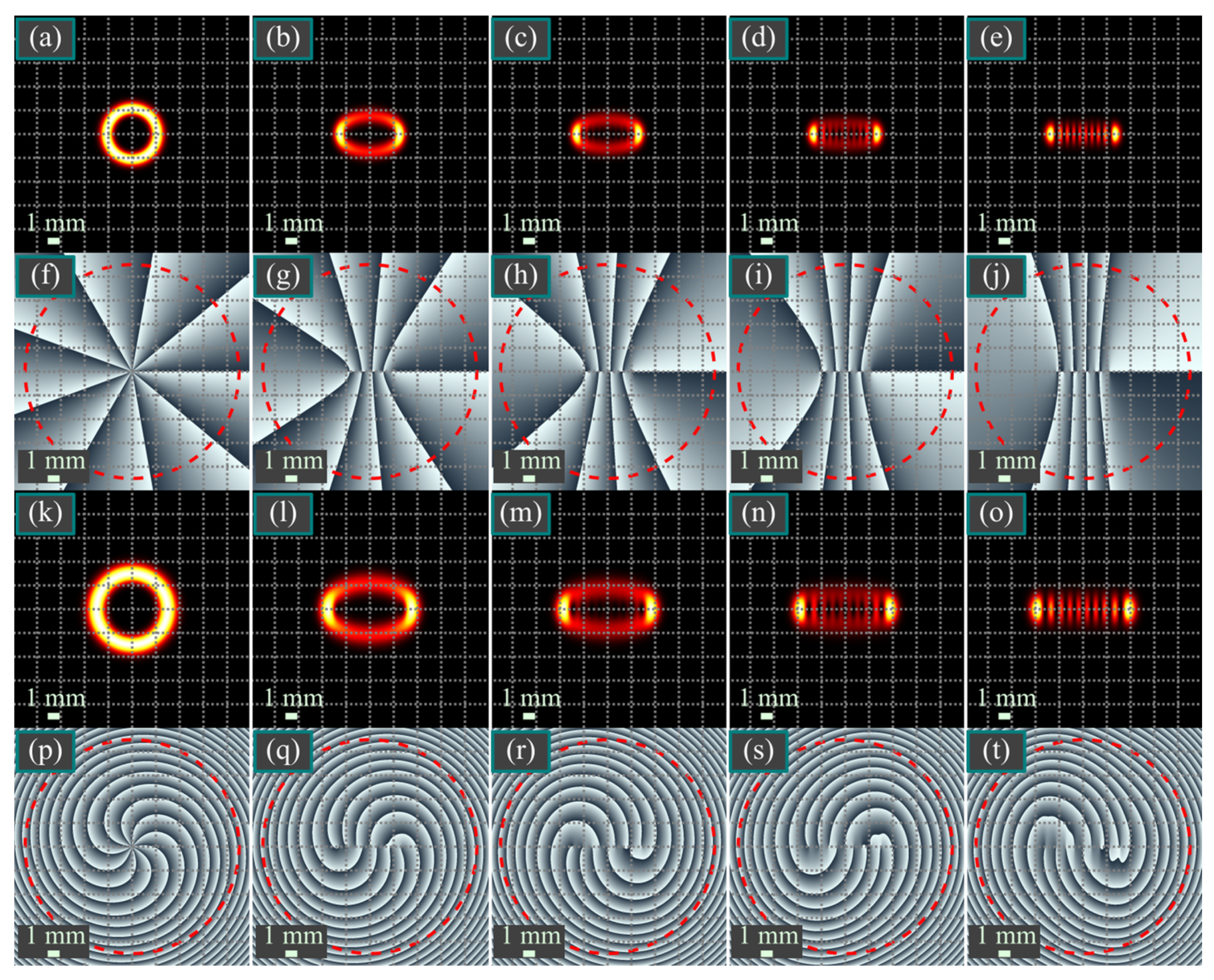
Figure 5 illustrates the intensity and phase distributions of propagation-invariant superpositions of the Laguerre–Gaussian beams (28) for different orders N (4, 6, 8, 10, 12) in the initial plane z = 0 and at the Rayleigh distance z = z0. Computation of the topological charge over the phase distributions from Figure 5 yielded the following values: 3.999935 (Figure 5f), 5.999776 (Figure 5g), 7.999475 (Figure 5h), 9.998990 (Figure 5i), 11.998284 (Figure 5j), 3.986310 (Figure 5p), 5.979236 (Figure 5q), 7.971959 (Figure 5r), 9.964446 (Figure 5s), and 11.956664 (Figure 5t). Thus, computation confirms that the TC is equal to N.
8. Conclusions
In this work, the following results have been obtained. For the known family of propagation-invariant vortex Hermite–Laguerre–Gaussian laser beams, which are finite superpositions of Hermite–Gaussian beams with a constant sum of indices of the Hermite polynomials n + m and whose intensity shape depends on the parameter θ, we have demonstrated theoretically and numerically that, for an arbitrary value θ from the half-interval (0, π/4], the topological charge of these beams is equal to n − m. If θ = 0, the topological charge of the Hermite–Laguerre–Gaussian beam is zero. For another type of propagation-invariant beams, called two-parametric vortex Hermite beams, which are also finite superpositions of the Hermite beams with a constant sum of indices n + m and with the partial amplitudes given by the binomial coefficients, we have shown theoretically and numerically that the topological charge is equal to the sum of indices n + m if both parameters are of the same sign, and equal to –(n + m) if the parameters are of different signs. We have also shown that if a propagation-invariant beam is a finite superposition of the Laguerre–Gaussian beams with the radial index p and with the azimuthal index l > 0, such that their combination 2p + l is constant, and if the amplitude multipliers are chosen as the binomial coefficients, then the topological charge of these beams is equal to 2p + l. This study has also revealed that the topological charge, which is one of the important characteristics of optical vortices along with the orbital angular momentum, is a quantity resistant to changing parameters of propagation-invariant beams. For instance, when the parameters θ and α of the Hermite–Laguerre–Gaussian beams are changed, the topological charge remains constant. The topological charge also remains unchanged upon the free-space propagation of beams. The obtained results will be useful for probing a weak-turbulence atmosphere by propagation-invariant vortex laser beams and for beam identification by measuring the beam topological charge, rather than the orbital angular momentum, since it remains constant at small beam distortions. The topological charge of vortex laser beams can be measured by using the Hartmann wavefront sensor. The simplest way to obtain the OAM of a laser beam is using a cylindrical lens.
Author Contributions
Conceptualization, V.V.K. and E.G.A.; methodology, V.V.K. and E.G.A.; software, A.A.K.; validation, V.V.K. and A.A.K.; formal analysis, V.V.K.; investigation, V.V.K., E.G.A. and A.A.K..; resources, V.V.K.; data curation, V.V.K.; writing—original draft preparation, V.V.K.; writing—review and editing, V.V.K. and E.G.A.; visualization, A.A.K.; supervision, V.V.K.; project administration, V.V.K.; funding acquisition, V.V.K. All authors have read and agreed to the published version of the manuscript.
Funding
This work was funded by the RUSSIAN SCIENCE FOUNDATION under grant No. 23-12-00236 (Theoretical background). This work was also performed within the State assignment of Federal Scientific Research Center “Crystallography and Photonics” of Russian Academy of Sciences (Simulation).
Institutional Review Board Statement
Not applicable.
Informed Consent Statement
Not applicable.
Data Availability Statement
Not applicable.
Conflicts of Interest
The authors declare no conflict of interest. The funders had no role in the design of the study; in the collection, analyses, or interpretation of data; in the writing of the manuscript; or in the decision to publish the results.
References
- Abramochkin, E.G.; Volostnikov, V.G. Generalized Gaussian beams. J. Opt. A Pure Appl. Opt. 2004, 6, S157–S161. [Google Scholar] [CrossRef]
- Abramochkin, E.; Razueva, E.; Volostnikov, V. General astigmatic transform of Hermite–Laguerre–Gaussian beams. J. Opt. Soc. Am. A 2010, 27, 2506–2513. [Google Scholar] [CrossRef]
- Deng, D.; Guo, Q.; Hu, W. Hermite–Laguerre–Gaussian beams in strongly nonlocal nonlinear media. J. Phys. B At. Mol. Opt. Phys. 2008, 41, 225402. [Google Scholar] [CrossRef]
- Xu, Y.Q.; Zhou, G.Q.; Wang, X.G. Nonparaxial propagation of Hermite–Laguerre–Gaussian beams in uniaxial crystal orthogonal to the optical axis. Chin. Phys. B 2013, 22, 064101. [Google Scholar] [CrossRef]
- Duan, K.; Lü, B. Propagation of Hermite–Laguerre–Gaussian beams through a paraxial optical ABCD system with rectangular hard-edged aperture. Opt. Commun. 2005, 250, 1–9. [Google Scholar] [CrossRef]
- Deng, D.; Guo, Q. Elegant Hermite–Laguerre–Gaussian beams. Opt. Lett. 2008, 33, 1225–1227. [Google Scholar] [CrossRef]
- Abramochkin, E.; Alieva, T. Closed-form expression for mutual intensity evolution of Hermite–Laguerre–Gaussian Schell-model beams. Opt. Lett. 2017, 42, 4032–4035. [Google Scholar] [CrossRef] [Green Version]
- Zhang, J.; Yu, X.; Chen, Y.; Huang, M.; Dai, X.; Liu, D. Generation of Hermite-Laguerre-Gaussian beams based on space-variant Pancharatnam Berry phase. Proc. SPIE 2018, 10964, 109645R. [Google Scholar] [CrossRef]
- Abramochkin, E.; Volostnikov, V. Spiral-type beams: Optical and quantum aspects. Opt. Commun. 1996, 125, 302–323. [Google Scholar] [CrossRef]
- Abramochkin, E.G.; Volostnikov, V.G. Modern optics of Gaussian Beams; Fizmatlit: Moscow, Russia, 2010; ISBN 978-5-9221-1216-1. (In Russian) [Google Scholar]
- Kotlyar, V.V.; Kovalev, A.A. Orbital angular momentum of paraxial propagation-invariant laser beams. J. Opt. Soc. Am. A 2022, 39, 1061–1065. [Google Scholar] [CrossRef]
- Zannotti, A.; Denz, C.; Alonso, M.A.; Dennis, M.R. Shaping caustics into propagation-invariant light. Nat. Commun. 2020, 11, 3597. [Google Scholar] [CrossRef] [PubMed]
- Soskind, M.; Soskind, R.; Soskind, Y. Shaping propagation invariant laser beams. Opt. Eng. 2015, 54, 111309. [Google Scholar] [CrossRef]
- Hansen, A.; Schultz, J.T.; Bigelow, N.P. Singular atom optics with spinor Bose–Einstein condensates. Optica 2016, 3, 355–361. [Google Scholar] [CrossRef]
- Wang, J.; Yang, J.Y.; Fazal, I.M.; Ahmed, N.; Yan, Y.; Huang, H.; Ren, Y.; Yue, Y.; Dolinar, S.; Tur, M.; et al. Terabit free-space data transmission employing orbital angular momentum multiplexing. Nat. Photon. 2012, 6, 488–496. [Google Scholar] [CrossRef]
- Torres, J.P. Multiplexing twisted light. Nat. Photon. 2012, 6, 420–422. [Google Scholar] [CrossRef]
- Xie, Z.; Lei, T.; Li, F.; Qiu, H.; Zhang, Z.; Wang, H.; Min, C.; Du, L.; Li, Z.; Yuan, X. Ultra-broadband on-chip twisted light emitter for optical communications. Light Sci. Appl. 2018, 7, 18001. [Google Scholar] [CrossRef] [Green Version]
- Sit, A.; Bouchard, F.; Fickler, R.; Gagnon-Bischoff, J.; Larocque, H.; Heshami, K.; Elser, D.; Peuntinger, C.; Günthner, K.; Heim, B.; et al. High-dimensional intracity quantum cryptography with structured photons. Optica 2017, 4, 1006–1010. [Google Scholar] [CrossRef] [Green Version]
- Sit, A.; Fickler, R.; Alsaiari, F.; Bouchard, F.; Larocque, H.; Gregg, P.; Yan, L.; Boyd, R.W.; Ramachandran, S.; Karimi, E. Quantum cryptography with structured photons through a vortex fiber. Opt. Lett. 2018, 43, 4108–4111. [Google Scholar] [CrossRef]
- Erhard, M.; Fickler, R.; Krenn, M.; Zeilinger, A. Twisted photons: New quantum perspectives in high dimensions. Light Sci. Appl. 2018, 7, 17146. [Google Scholar] [CrossRef] [Green Version]
- Mathis, A.; Courvoisier, F.; Froehly, L.; Furfaro, L.; Jacquot, M.; Lacourt, P.A.; Dudley, J.M. Micromachining along a curve: Femtosecond laser micromachining of curved profiles in diamond and silicon using accelerating beams. Appl. Phys. Lett. 2012, 101, 071110. [Google Scholar] [CrossRef] [Green Version]
- Courvoisier, F.; Stoian, R.; Couairon, A. Ultrafast laser micro-and nano-processing with nondiffracting and curved beams. Opt. Laser Technol. 2016, 80, 125–137. [Google Scholar] [CrossRef]
- Hell, S.W.; Wichmann, J. Breaking the diffraction resolution limit by stimulated emission: Stimulated-emission-depletion fluorescence microscopy. Opt. Lett. 1994, 19, 780–782. [Google Scholar] [CrossRef] [PubMed]
- Willig, K.I.; Harke, B.; Medda, R.; Hell, S.W. STED microscopy with continuous wave beams. Nat. Methods 2007, 4, 915–918. [Google Scholar] [CrossRef]
- Fahrbach, F.O.; Simon, P.; Rohrbach, A. Microscopy with self-reconstructing beams. Nat. Photon. 2010, 4, 780–785. [Google Scholar] [CrossRef]
- Vettenburg, T.; Dalgarno, H.I.; Nylk, J.; Coll-Lladó, C.; Ferrier, D.E.; Čižmár, T.; Gunn-Moore, F.J.; Dholakia, K. Light-sheet microscopy using an Airy beam. Nat. Methods 2014, 11, 541–544. [Google Scholar] [CrossRef] [Green Version]
- Dholakia, K.; Čižmár, T. Shaping the future of manipulation. Nat. Photon. 2011, 5, 335–342. [Google Scholar] [CrossRef]
- Woerdemann, M.; Alpmann, C.; Esseling, M.; Denz, C. Advanced optical trapping by complex beam shaping. Laser Photon. Rev. 2013, 7, 839–854. [Google Scholar] [CrossRef]
- Volyar, A.; Abramochkin, E.; Egorov, Y.; Bretsko, M.; Akimova, Y. Fine structure of perturbed Laguerre–Gaussian beams: Hermite–Gaussian mode spectra and topological charge. Appl. Opt. 2020, 59, 7680–7687. [Google Scholar] [CrossRef]
- Volyar, A.; Abramochkin, E.; Akimova, Y.; Bretsko, M. Super bursts of the orbital angular momentum in astigmatic-invariant structured LG beams. Opt. Lett. 2022, 47, 5537–5540. [Google Scholar] [CrossRef]
- Volyar, A.; Abramochkin, E.; Akimova, Y.; Bretsko, M. Control of the orbital angular momentum via radial numbers of structured Laguerre–Gaussian beams. Opt. Lett. 2022, 47, 2402–2405. [Google Scholar] [CrossRef]
- Kotlyar, V.V.; Kovalev, A.A.; Porfirev, A.P. Vortex Hermite–Gaussian laser beams. Opt. Lett. 2015, 40, 701–704. [Google Scholar] [CrossRef] [PubMed]
- Berry, M.V. Optical vortices evolving from helicoidal integer and fractional phase steps. J. Opt. A Pure Appl. Opt. 2004, 6, 259–268. [Google Scholar] [CrossRef]
- Prudnikov, A.P.; Brychkov, Y.A.; Marichev, O.I. Integrals and Series. Volume 2: Special Functions; Gordon and Breach: New York, NY, USA, 1986; ISBN 2-88124-097-6. [Google Scholar]
- Prudnikov, A.P.; Brychkov, Y.A.; Marichev, O.I. Integrals and Series. Volume 1: Elementary Functions; Gordon and Breach: New York, NY, USA, 1986; ISBN 2-88124-097-6. [Google Scholar]
- Kotlyar, V.; Kovalev, A.; Kozlova, E.; Savelyeva, A.; Stafeev, S. Geometric Progression of Optical Vortices. Photonics 2022, 9, 407. [Google Scholar] [CrossRef]
Figure 1.
Intensity (a–e,k–o) and phase (f–j,p–t) distributions of the Hermite–Laguerre–Gaussian beams (12) in the initial plane z = 0 (a–j) and at the Rayleigh distance z = z0 (k–t) for different θ values. Computation parameters: wavelength λ = 532 nm, waist radius of the Gaussian beam w0 = 1 mm, the beam order (orders of the Hermite polynomials) (n, m) = (5, 3), values of the parameter θ: 0 (a,f,k,p), π/16 (b,g,l,q), π/8 (c,h,m,r), 3π/16 (d,i,n,s), π/4 (e,j,o,t). Scale mark in each figure denotes 1 mm. The red dashed circles in the phase distributions are the circles over which the topological charge was computed. Black and white colors denote, respectively, the phase of 0 and π (f), or 0 and 2π (g–j,p–t).

Figure 2.
Intensity (a–e,k–o) and phase (f–j,p–t) distributions of the Hermite–Laguerre–Gaussian beams (12) in the initial plane z = 0 (a–j) and at the Rayleigh distance z = z0 (k–t) for different values θ. Computation parameters: wavelength λ = 532 nm, waist radius of the Gaussian beam w0 = 1 mm, beam order (orders of the Hermite polynomials) (n, m) = (2, 7), values of the parameter θ: 0 (a,f,k,p), π/16 (b,g,l,q), π/8 (c,h,m,r), 3π/16 (d,i,n,s), π/4 (e,j,o,t). Scale mark in each figure denotes 1 mm. The red dashed circles in the phase distributions are the circles over which the topological charge was computed. Black and white colors denote, respectively, the phase of 0 and π (f), or 0 and 2π (g–j,p–t).

Figure 3.
Intensity (a–e,k–o) and phase (f–j,p–t) distributions of the Hermite–Laguerre–Gaussian beams (12) in the initial plane z = 0 (a–j) and at the Rayleigh distance z = z0 (k–t) for different values of the parameter α. Computation parameters: wavelength λ = 532 nm, waist radius of the Gaussian beam w0 = 1 mm, beam order (orders of the Hermite polynomials) (n, m) = (5, 3), value of the parameter θ: θ = π/8, values of the parameter α: 1 (a,f,k,p), 0.8 (b,g,l,q), 0.6 (c,h,m,r), 0.4 (d,I,n,s), 0.2 (e,j,o,t). Scale mark in each figure denotes 1 mm. The red dashed circles in the phase distributions are the circles over which the topological charge was computed. Black and white colors denote, respectively, the phase of 0 and 2π (f–j,p–t).

Figure 4.
Intensity (a–e,k–o) and phase (f–j,p–t) distributions of the two-parametric vortex Hermite beams (21) in the initial plane z = 0 (a–j) and at the Rayleigh distance z = z0 (k–t) for different values of the parameters t and τ. Computation parameters: wavelength λ = 532 nm, waist radius of the Gaussian beam w0 = 1 mm, beam order (orders of the Hermite polynomials) (n, m) = (2, 7), values of the parameters (t, τ): (0.7, 0.7) (a,f,k,p), (0.7, 0.4) (b,g,l,q), (0.7, –0.3) (c,h,m,r), (0.7, 0.2) (d,i,n,s), (0.7, –0.1) (e,j,o,t). Scale mark in each figure denotes 1 mm. The red dashed circles in the phase distributions are the circles over which the topological charge was computed. Black and white colors denote, respectively, the phase of 0 and 2π (f–j,p–t).

Figure 5.
Intensity (a–e,k–o) and phase (f–j,p–t) distributions of propagation-invariant superpositions of the Laguerre–Gaussian beams (28) in the initial plane z = 0 (a–j) and at the Rayleigh distance z = z0 (k–t) for different beam orders N. Computation parameters: wavelength λ = 532 nm, waist radius of the Gaussian beam w0 = 1 mm, beam order N = 4 (a,f,k,p), 6 (b,g,l,q), 8 (c,h,m,r), 10 (d,i,n,s), 12 (e,j,o,t). Scale mark in each figure denotes 1 mm. The red dashed circles in the phase distributions are the circles over which the topological charge was computed.

Disclaimer/Publisher’s Note: The statements, opinions and data contained in all publications are solely those of the individual author(s) and contributor(s) and not of MDPI and/or the editor(s). MDPI and/or the editor(s) disclaim responsibility for any injury to people or property resulting from any ideas, methods, instructions or products referred to in the content. |
© 2023 by the authors. Licensee MDPI, Basel, Switzerland. This article is an open access article distributed under the terms and conditions of the Creative Commons Attribution (CC BY) license (https://creativecommons.org/licenses/by/4.0/).
Share and Cite
MDPI and ACS Style
Kotlyar, V.V.; Kovalev, A.A.; Abramochkin, E.G. Topological Charge of Propagation-Invariant Laser Beams. Photonics 2023, 10, 915. https://doi.org/10.3390/photonics10080915
AMA Style
Kotlyar VV, Kovalev AA, Abramochkin EG. Topological Charge of Propagation-Invariant Laser Beams. Photonics. 2023; 10(8):915. https://doi.org/10.3390/photonics10080915
Chicago/Turabian StyleKotlyar, Victor V., Alexey A. Kovalev, and Eugeny G. Abramochkin. 2023. "Topological Charge of Propagation-Invariant Laser Beams" Photonics 10, no. 8: 915. https://doi.org/10.3390/photonics10080915
Note that from the first issue of 2016, this journal uses article numbers instead of page numbers. See further details here.