Impact of Lorentz Violation Models on Exoplanets’ Dynamics

Abstract

Many exoplanets have been detected by the radial velocity method, according to which the motion of a binary system around its center of mass can produce a periodical variation of the Doppler effect of the light emitted by the host star. These variations are influenced by both Newtonian and non-Newtonian perturbations to the dominant inverse-square acceleration; accordingly, exoplanetary systems lend themselves to testing theories of gravity alternative to general relativity. In this paper, we consider the impact of the Standard Model Extension (a model that can be used to test all possible Lorentz violations) on the perturbation of radial velocity and suggest that suitable exoplanets’ configurations and improvements in detection techniques may contribute to obtaining new constraints on the model parameters.

1. Introduction

After the first detection of a planet orbiting a main sequence star [1], thousands of exoplanets have been detected using different techniques, such as radial velocity, transit photometry and timing, pulsar timing, microlensing and astrometry; indeed, each of these techniques is sensitive to the specific properties of the planetary systems, unavoidably leading to selection effects in the detection process [2,3].

Radial velocity (RV) is a powerful tool that is used not only in the search for exoplanets but, more generally, to discover an invisible celestial object gravitationally bound to another one. The underlying idea is the following: by accurately observing the light spectrum of the visible body, it is possible to detect periodical variations in the wavelength due to the Doppler effect determined by the motion of the system around the center of mass. This is the projection of the velocity vector onto the line of sight. Obviously, in an exoplanetary system, the visible body is the host star, while the invisible one is the planet, but a similar approach can be applied also to a binary system made of a main sequence star and a white dwarf, a neutron star, or a black hole.

In a previous work [4], one of the authors introduced a comprehensive approach to obtain the impact of post-Keplerian (pK) corrections to the dominant Newtonian inverse-square acceleration on radial velocity; in particular, they can be of both Newtonian and non-Newtonian origin, for instance, deriving from models of gravity alternative to general relativity (GR). In fact, on the one hand, we know that more than 100 years after its publication, GR remains the best model to describe gravitation interaction, as its predictions were verified with great accuracy [5]. However, there are challenges coming from the observation of the universe at very large scales [6], and in addition, there are known problems when one tries to reconcile GR with the standard model of particle physics. Consequently, it is expected that GR could represent a suitable limit of a more general theory, which we still ignore. As a consequence, there are various and sound motivations to try to extend Einstein’s theory; summaries of diverse modified gravity models can be found in the review papers [7,8,9,10,11,12,13,14,15,16,17].

In this context, the role of Lorentz symmetry is quite relevant; in fact, it represents a fundamental property of the mathematical model of spacetime at the basis of GR. It is useful to remember that the bounds of the violation of Lorentz invariance were obtained from the binary neutron star (BNS) merger [18]. Nonetheless, it would be desirable to obtain constraints from different systems, such as exoplanets.

Thus, the search for a more fundamental theory brings about a careful investigation of possible Lorentz violations (LV). The Standard Model Extension (SME) is a framework that can be used to experimentally test all possible Lorentz violations [19,20,21,22,23,24,25,26,27,28].

The purpose of this paper is to calculate the perturbation of the radial velocities within the SME, in order to evaluate their impact on the current observation of exoplanets. More specifically, we wish to explore the potential that such a method may have in constraining the relevant LV-parameters in light of the current and expected accuracies in measuring exoplanetary RVs. In particular, we calculate the instantaneous and orbit-averaged radial velocity variations; in fact, the latter are very useful, since there are data records covering many orbital revolutions for this kind of system.

The paper is organized as follows: we define the impact of the SME coefficients on the system dynamics in Section 2, and we calculate, to the lowest order in eccentricity, the perturbation of the radial velocity in Section 3; the discussion and conclusion are presented in Section 4.

2. Definition of the Perturbing Acceleration

The SME is based on Riemann–Cartan spacetime; in particular (see, e.g., Bailey and Kostelecký [21]), if we focus on the pure-gravity sector, the relevant equation of motion can be derived from a Lagrangian in the form $L=L_{\mathrm{LI}}+L_{\mathrm{LV}}$, where $L_{\mathrm{LI}}$ and $L_{\mathrm{LV}}$ refer to the Lorentz-inviariant and Lorentz-violating terms, respectively. In the limit of Riemannian spacetime, the pure-gravity sector Lagrangian turns out to be the usual Einstein–Hilbert action $L_{\mathrm{LI}}=\sqrt{-g}(R-2\mathsf{\Lambda })/16\pi G$, where G is the Newtonian constant of gravitation, R is the Ricci scalar, g is the metric determinant, and $\mathsf{\Lambda }$ is the cosmological constant. Then, the Lorentz-violating Lagrangian turns out to be [21,23]:

$$L_{\mathrm{LV}}=\frac{\sqrt{-g}}{16\pi G}\left(-uR+s^{\mu \nu }{R}_{\mu \nu }^{\mathrm{T}}+t^{\kappa \lambda \mu \nu }{C}_{\kappa \lambda \mu \nu }\right).$$

(1)

Notice that it is possible to consider additional contributions in the action (1), deriving from a nonminimal SME expansion (see, e.g., Kostelecký and Russell [19], Bailey et al. [29], Kostelecký and Mewes [30], Bailey and Havert [31]). In the above expression, $R_{\mu \nu }^{\mathrm{T}}$ is the trace-free Ricci tensor, and $C_{\kappa \lambda \mu \nu }$ is the Weyl conformal tensor. The u, $s^{\mu \nu }$, and $t^{\kappa \lambda \mu \nu }$ objects are Lorentz-violating fields; more precisely, they violate the particle local Lorentz invariance and the diffeomorphism, while the observer local Lorentz invariance is maintained [23]. The post-Newtonian analysis of the SME equations for the pure-gravity sector, as discussed by Bailey and Kostelecký [21], show that the relevant terms in the metric that describe the leading observable effects are determined by the components of a trace-free matrix ${\overline{s}}^{\mu \nu }$, which are the (rescaled) vacuum expectation values of $s^{\mu \nu }$. It is relevant to point out that while ${\overline{s}}^{\mu \nu }$ is observer Lorentz-invariant, it turns out to be particle Lorentz-violating [23]. Accordingly, it is important to specify the observer reference system that we are using. To begin with, we refer to the reference frame at rest with the binary system barycenter. In this frame, according to Bailey and Kostelecký [21], Bailey [32], it is possible to write the acceleration acting on a test particle in terms of the gravitoelectric field ${\mathit{a}}_{GE}={\mathit{E}}_G$, where

$$E_G^j=-\frac{GM}{r^2}\left[{\widehat{r}}^j\left(1+\frac{3}{2}{\overline{s}}^{00}+\frac{3}{2}{\overline{s}}^{kl}{\widehat{r}}^k{\widehat{r}}^l\right)-{\overline{s}}^{jk}{\widehat{r}}^k\right].$$

(2)

In the above expression, M is the mass of the primary, $\mathit{r}$ is the position vector with respect to the primary, and $\widehat{\mathbf{r}}$ is the unit vector, ${\displaystyle \widehat{\mathbf{r}}=\frac{\mathit{r}}{r}}$. Equation (2) can be written in the form

$${\mathit{E}}_G={\mathit{E}}_{G,N}+\Delta \mathit{E},$$

(3)

where ${\mathit{E}}_{G,N}$ is the Newtonian field, and $\Delta \mathit{E}$ is the perturbation, which can be written as

$$\Delta E^i=-\frac{GM}{r^2}\left(\frac{3}{2}{\overline{s}}^{00}+\frac{3}{2}{\overline{s}}^{kl}{\widehat{r}}^k{\widehat{r}}^l\right){\widehat{r}}^i+\frac{GM}{r^2}{\overline{s}}^{ik}{\widehat{r}}^k.$$

(4)

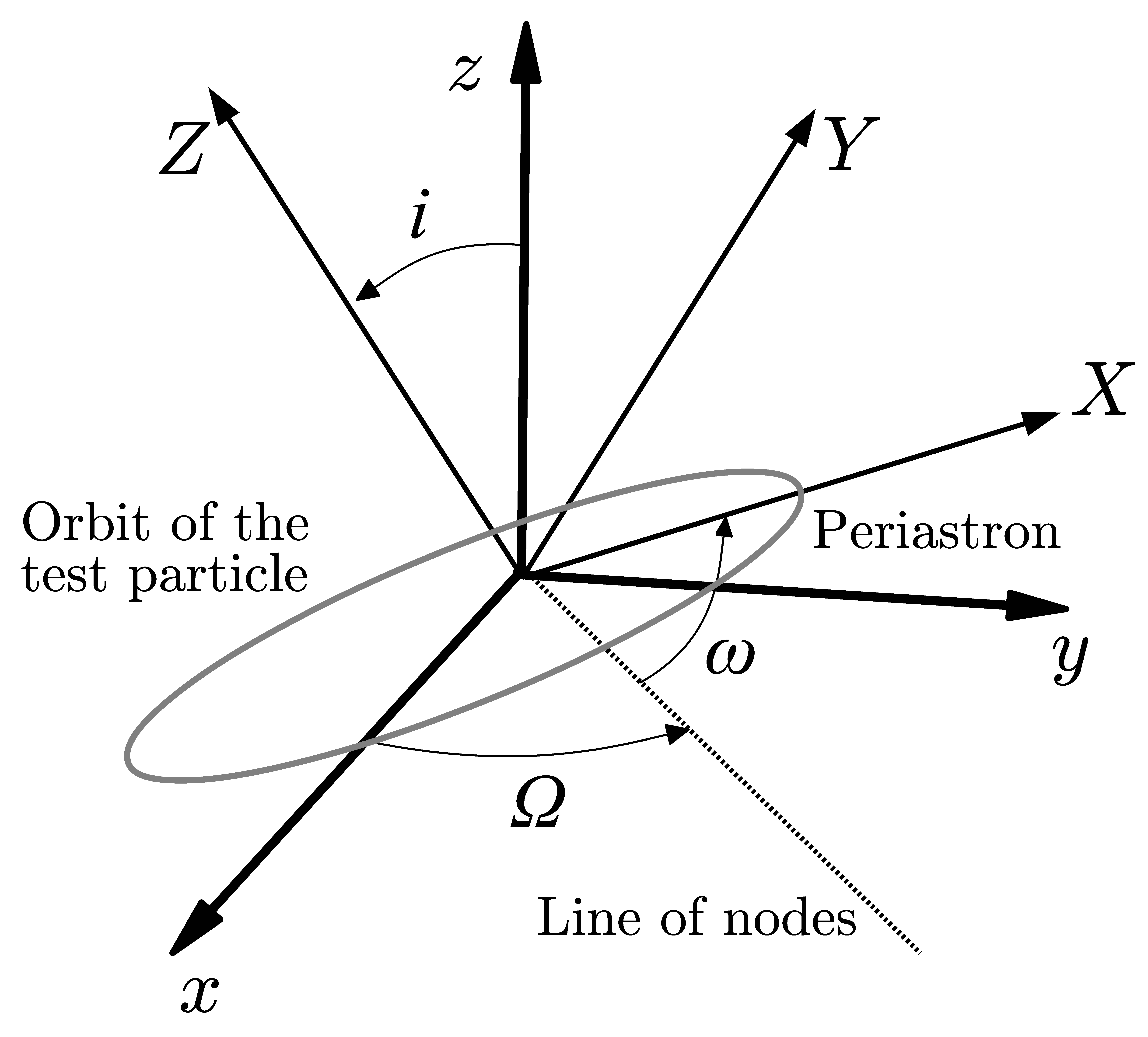
In order to evaluate the impact of the above acceleration on the motion of a planet, which can be thought of as a test particle, let us start by suitably parameterizing its unperturbated motion (in doing this, we follow the approach described in Ref. [21]). We first define a reference frame, with its origin in the focus of the planet orbit; in this frame, we consider a set of Cartesian coordinates $\{x,y,z\}$, where z is directed along the line of sight toward the Earth. An arbitrary configuration of the test particle orbit is shown in Figure 1; besides the already mentioned Cartesian coordinate system $\{x,y,z\}$, with unit vectors ${\mathit{u}}_x,{\mathit{u}}_y,$ and ${\mathit{u}}_z$, we introduce another Cartesian coordinate system $\{X,Y,Z\}$, with the same origin and unit vectors ${\mathit{u}}_X,{\mathit{u}}_Y,$ and ${\mathit{u}}_Z$. The orbital plane is the $XY$ plane, and we denote with $\Omega$ the angle between the x axis and the line of the nodes, while the angle between the z and Z axes is called i. The periastron is along the X axis, and we denote by $\omega$ the argument of the periastron, i.e., the angle between the line of nodes and the X axis. The following relations hold between the unit vectors of the two Cartesian coordinate systems (see, e.g., Bertotti et al. [33]):

$$\begin{array}{ccc}\hfill {\mathit{u}}_X& =& \left(cos\omega cos\Omega -sin\omega cosisin\Omega \right){\mathit{u}}_x+\left(cos\omega sin\Omega +sin\omega cosicos\Omega \right){\mathit{u}}_y+sin\omega sini{\mathit{u}}_z\hfill \\ \hfill {\mathit{u}}_Y& =& \left(-sin\omega cos\Omega -cos\omega cosisin\Omega \right){\mathit{u}}_x+\left(-sin\omega sin\Omega +cos\omega cosicos\Omega \right){\mathit{u}}_y+cos\omega sini{\mathit{u}}_z\hfill \\ \hfill {\mathit{u}}_Z& =& sinisin\Omega {\mathit{u}}_x-sinicos\Omega {\mathit{u}}_y+cosi{\mathit{u}}_z.\hfill \end{array}$$

(5)

In what follows, for direct comparison with previous works (see, e.g., Bailey and Kostelecký [21]), we use the following notation for the above vectors:

$${\mathit{u}}_X\to \mathit{P},{\mathit{u}}_Y\to \mathit{Q},{\mathit{u}}_Z\to \mathit{N}.$$

(6)

Notice that $\mathit{P}$ is directed from the focus (and origin of the coordinate system) to the periastron; $\mathit{N}$ is orthogonal to the orbital plane. The unit vectors $\mathit{P},\mathit{Q},$ and $\mathit{N}$ depend on the orbital elements only. Let $\mathit{X}$ denote the position vector of the test particle, which in the orbital plane can be written as

$$\mathit{X}=r\left(f\right)cosf\mathit{P}+r\left(f\right)sinf\mathit{Q},$$

(7)

where the Keplerian ellipse, parameterized by the true anomaly f, is written as

$$r\left(f\right)=\frac{a\left(1-e^2\right)}{1+ecosf}$$

(8)

in terms of the semi-major axis a and eccentricity e.

Along the orbit, we define the radial vector $\mathit{R}$

$$\mathit{R}=cosf\mathit{P}+sinf\mathit{Q},$$

(9)

and the transverse vector $\mathit{T}$

$$\mathit{T}=-sinf\mathit{P}+cos\mathit{Q}.$$

(10)

The perturbing acceleration (4) must be evaluated along the orbit; so, $\widehat{\mathbf{r}}=\mathit{R}$. Accordingly, using the definitions (9), (10), the perturbing acceleration can be written in the form

$$\Delta E^i=-\frac{GM}{r^2}{\alpha }_1{\widehat{r}}^i+\frac{GM}{r^2}{\overline{s}}^{ik}{\widehat{r}}^k,$$

(11)

where

$${\alpha }_1=\frac{3}{2}\left[{\overline{s}}^{00}+{\overline{s}}^{PP}{cos}^{2}f+{\overline{s}}^{QQ}{sin}^{2}f+2{\overline{s}}^{PQ}sinfcosf\right],$$

(12)

with

$${\overline{s}}^{PP}={\overline{s}}^{kl}{\widehat{P}}^k{\widehat{P}}^l,{\overline{s}}^{QQ}={\overline{s}}^{kl}{\widehat{Q}}^k{\widehat{Q}}^l,{\overline{s}}^{PQ}={\overline{s}}^{kl}{\widehat{P}}^k{\widehat{Q}}^l.$$

(13)

Notice that ${\overline{s}}^{PP}$, ${\overline{s}}^{QQ}$, and ${\overline{s}}^{PQ}$ depend on the orbital elements only.

Now, we can calculate the radial, transverse, and normal components of the perturbing acceleration (11). We obtain

$$\begin{array}{cc}\hfill E_r& =\Delta \mathit{E}·\mathit{R}=-\frac{GM}{r^2}\left[\frac{3}{2}{\overline{s}}^{00}+\frac{1}{2}\left({\overline{s}}^{PP}{cos}^{2}f+{\overline{s}}^{QQ}{sin}^{2}f+2{\overline{s}}^{PQ}sinfcosf\right)\right],\hfill \end{array}$$

(14)

$$\begin{array}{cc}\hfill E_t& =\Delta \mathit{E}·\mathit{T}=\frac{GM}{r^2}\left[cosfsinf\left({\overline{s}}^{QQ}-{\overline{s}}^{PP}\right)+\left({cos}^{2}f-{sin}^{2}f\right){\overline{s}}^{PQ}\right],\hfill \end{array}$$

(15)

$$\begin{array}{cc}\hfill E_n& =\Delta \mathit{E}·\mathit{N}=\frac{GM}{r^2}\left[cosf{\overline{s}}^{NP}+sinf{\overline{s}}^{NQ}\right],\hfill \end{array}$$

(16)

where

$${\overline{s}}^{NP}={\overline{s}}^{kl}{\widehat{N}}^k{\widehat{P}}^l,{\overline{s}}^{NQ}={\overline{s}}^{kl}{\widehat{N}}^k{\widehat{Q}}^l.$$

(17)

Given the components of the perturbing acceleration, we may write the Gauss equations for the variations of the semi-major axis a, the eccentricity e, the inclination i, the longitude of the ascending node $\Omega$, and the argument of pericenter $\omega$:

$$\begin{array}{cc}\hfill \frac{\mathrm{d}a}{\mathrm{d}t}& =\frac{2}{n_{\mathrm{b}}\sqrt{1-e^2}}\left[e{E}_{r}sinf+E_t\left(\frac{p}{r}\right)\right],\hfill \end{array}$$

(18)

$$\begin{array}{cc}\hfill \frac{\mathrm{d}e}{\mathrm{d}t}& =\frac{\sqrt{1-e^2}}{n_{\mathrm{b}}a}\left\{E_{r}sinf+E_t\left[cosf+\frac{1}{e}\left(1-\frac{r}{a}\right)\right]\right\},\hfill \end{array}$$

(19)

$$\begin{array}{cc}\hfill \frac{\mathrm{d}i}{\mathrm{d}t}& =\frac{1}{n_{\mathrm{b}}a\sqrt{1-e^2}}{E}_n\left(\frac{r}{a}\right)cos(\omega +f),\hfill \end{array}$$

(20)

$$\begin{array}{cc}\hfill \frac{\mathrm{d}\Omega }{\mathrm{d}t}& =\frac{1}{n_{\mathrm{b}}asini\sqrt{1-e^2}}{E}_n\left(\frac{r}{a}\right)sin(\omega +f),\hfill \end{array}$$

(21)

$$\begin{array}{cc}\hfill \frac{\mathrm{d}\omega }{\mathrm{d}t}& =-cosi\frac{\mathrm{d}\Omega }{\mathrm{d}t}+\frac{\sqrt{1-e^2}}{n_{\mathrm{b}}ae}\left[-E_{r}cosf+E_t\left(1+\frac{r}{p}\right)sinf\right].\hfill \end{array}$$

(22)

In the above equations, $n_{\mathrm{b}}=2\pi /T$ is the Keplerian mean motion1, T is the test particle’s orbital period, and $p=a\left(1-e^2\right)$ is the semilatus rectum.

In summary, in order to calculate the variation of orbital elements, we must evaluate the perturbing acceleration onto the unperturbed Keplerian ellipse; then, it must be inserted into Equations (18)–(22). Then, we must average over one orbital period T. To this end, the following relation

$$dt=\frac{{(1-e^2)}^{3/2}}{n_{\mathrm{b}}{(1+ecosf)}^2}df$$

(23)

is used.

3. The Method of Radial Velocity

As discussed by Iorio [4], the presence of a perturbing acceleration, whatever its origin (Newtonian or non-Newtonian), modifies the velocity vector $\mathbf{v}$ of the motion of the test particle relative to its primary.2 Namely (see also Casotto [34]), the instantaneous changes $\Delta {\mathrm{v}}_R,\Delta {\mathrm{v}}_T,$ and $\Delta {\mathrm{v}}_N$ of the radial, transverse, and out-of-plane components ${\mathrm{v}}_R,{\mathrm{v}}_T,$ and ${\mathrm{v}}_N$ are

$$\begin{array}{cc}\hfill \Delta {\mathrm{v}}_R\left(f\right)=& -\frac{n_{\mathrm{b}}asinf}{\sqrt{1-e^2}}\left[\frac{e}{2a}\Delta a\left(f\right)+\frac{a}{r\left(f\right)}\Delta e\left(f\right)\right]-\frac{n_{\mathrm{b}}{a}^3}{r^2\left(f\right)}\Delta \mathcal{M}\left(f\right)-\hfill \\ & -\frac{n_{\mathrm{b}}{a}^2}{r\left(f\right)}\sqrt{1-e^2}\left[cosi\Delta \Omega \left(f\right)+\Delta \omega \left(f\right)\right],\hfill \end{array}$$

(24)

$$\begin{array}{cc}\hfill \Delta {\mathrm{v}}_T\left(f\right)=& -\frac{n_{\mathrm{b}}a\sqrt{1-e^2}}{2r\left(f\right)}\Delta a\left(f\right)+\frac{n_{\mathrm{b}}a\left(e+cosf\right)}{{\left(1-e^2\right)}^{3/2}}\Delta e\left(f\right)+\frac{n_{\mathrm{b}}aesinf}{\sqrt{1-e^2}}\left[cosi\Delta \Omega \left(f\right)+\Delta \omega \left(f\right)\right],\hfill \end{array}$$

(25)

$$\begin{array}{cc}\hfill \Delta {\mathrm{v}}_N\left(f\right)=& \frac{n_{\mathrm{b}}a}{\sqrt{1-e^2}}\left[\left(cosu+ecos\omega \right)\Delta i\left(f\right)+\left(sinu+esin\omega \right)sini\Delta \Omega \left(f\right)\right].\hfill \end{array}$$

(26)

In the above equation, there are the instantaneous changes of the Keplerian orbital elements $\Delta a\left(f\right),\Delta e\left(f\right),\Delta i\left(f\right),\Delta \Omega \left(f\right),$ and $\Delta \omega \left(f\right)$; they can be calculated using the general relation

$$\Delta \kappa \left(f\right)={\int }_{f_0}^f\frac{\mathrm{d}\kappa }{\mathrm{d}t}\frac{\mathrm{d}t}{\mathrm{d}{f}^{\prime }}d{f}^{{}^{\prime }},\kappa =a,e,i,\Omega ,\omega ,$$

(27)

where the time derivatives can be obtained from the Gauss Equations (18)–(22) and $\frac{dt}{d{f}^{\prime }}$ from Equation (23), and $f_0$ is the expression of the true anomaly at a given epoch.

The variation $\Delta \mathcal{M}$ of the mean anomaly $\mathcal{M}$ can be calculated as in Iorio [35]. Care must be taken for the latter quantity, since the possible change in the mean motion $n_{\mathrm{b}}$ can influence the mean anomaly variation $\Delta \mathcal{M}$ [4]. In particular, this may happen when the perturbing acceleration provokes a variation in the semimajor axis. As shown by Bailey and Kostelecký [21], this is not the case for the modified gravity models with which we are dealing.

Then, it is possible to obtain the instantaneous change experienced by the radial velocity by taking the z component of the perturbation of the relative velocity ${\displaystyle \Delta \mathbf{v}=\Delta {\mathrm{v}}_R\mathit{R}+\Delta {\mathrm{v}}_T\mathit{T}+\Delta {\mathrm{v}}_N\mathit{N}}$. Accordingly, we obtain

$$\begin{array}{cc}\hfill \Delta {\mathrm{v}}_z\left(f\right)=& -\frac{n_{\mathrm{b}}sini\left(ecos\omega +cosu\right)}{2\sqrt{1-e^2}}\Delta a\left(f\right)+\hfill \\ \hfill & +\frac{n_{\mathrm{b}}asini\left\{4cos\left(2f+\omega \right)+e\left[-cos\left(f-\omega \right)+4cosu+cos\left(3f+\omega \right)\right]\right\}}{4{\left(1-e^2\right)}^{3/2}}\Delta e\left(f\right)+\hfill \\ \hfill & +\frac{n_{\mathrm{b}}acosi\left(ecos\omega +cosu\right)}{\sqrt{1-e^2}}\Delta i\left(f\right)-\frac{n_{\mathrm{b}}asini\left(esin\omega +sinu\right)}{\sqrt{1-e^2}}\Delta \omega \left(f\right)-\hfill \\ \hfill & -\frac{n_{\mathrm{b}}a{\left(1+ecosf\right)}^{2}sinisinu}{{\left(1-e^2\right)}^2}\Delta \mathcal{M}\left(f\right),\hfill \end{array}$$

(28)

where $u\doteq \omega +f$ is the argument of latitude.

Using Equation (28), we can calculate the net change of the radial velocity over an orbital period, namely

$$〈\Delta {\mathrm{v}}_z〉=\frac{1}{T}\underset{f_0}{\overset{f_0+2\pi }{\int }}\frac{dt}{df}\Delta {\mathrm{v}}_{z}df.$$

(29)

The explicit expression of $〈\Delta {\mathrm{v}}_z〉$ can be calculated, but it will not be displayed here, since it is quite unmanageable; rather, to evaluate its magnitude, we perform an expansion in powers of the eccentricity e and write the lowest order terms. Accordingly, we obtain

$$〈\Delta {\mathrm{v}}_z〉\simeq \frac{a}{T}\left(c_0+c_{1}e\right),$$

(30)

where

$$\begin{array}{cc}\hfill c_0=\frac{\pi }{2}\{& 2cosi\left[s_{NP}sin{f}_0-s_{NQ}cos{f}_0\right]+\hfill \\ \hfill & +sinicos(f_0+\omega )[3(s_{PP}-s_{QQ})cos\left(2f_0\right)+\hfill \\ \hfill & +2\left(6s_{00}+s_{PP}+s_{QQ}+3s_{PQ}sin\left(2f_0\right)\right)\left]\right\},\hfill \end{array}$$

(31)

and

$$\begin{array}{cc}\hfill c_1=\frac{\pi }{8}\{& 8cosicos{f}_0\left[s_{NQ}cos{f}_0-s_{NP}sin{f}_0\right]+\hfill \\ \hfill & +sini[9(s_{PP}-s_{QQ})cos(2f_0-\omega )+14(6s_{00}+s_{PP}+s_{QQ})cos\left(\omega \right)+\hfill \\ \hfill & +2(18s_{00}+7s_{PP}-s_{QQ})cos(2f_0+\omega )+3(s_{PP}-s_{QQ})cos(4f_0+\omega )+\hfill \\ \hfill & +2s_{PQ}\left(9sin(2f_0-\omega )+8sin(2f_0+\omega )+3sin(4f_0+\omega )\right)\left]\right\}.\hfill \end{array}$$

(32)

The above expressions suggest there is a non null net change also at the zeroth order in the eccentricity. We notice that the change in the radial velocity can be expressed in the form

$$〈\Delta {\mathrm{v}}_z〉\simeq v_m\Delta S,$$

(33)

where $v_m$ is the mean orbital speed, and $\Delta S$ is a factor that is linear depending on the elements of the Lorentz-violating matrix ${\overline{s}}^{\mu \nu }$; in addition, it depends on the (bounded) trigonometric function of the angular orbital elements. We see from the expressions above that the effect of the Lorentz-violating terms is enhanced in rapidly rotating systems, which appear to be ideal candidates for observing such perturbations. In addition, we notice that for rapidly rotating systems, data covering many orbital revolutions are available.

4. Discussion and Conclusions

As we showed above, the presence of Lorentz-violating terms produces a variation in the radial velocity that can be written (see Equation (33)) in the form:

$$\mathrm{mean}\mathrm{orbital}\mathrm{speed}\times \mathrm{perturbation}.$$

We emphasize that even though we refer to exoplanetary systems, these results can be applied to any gravitationally bound binary system.

The elements of the Lorentz-violating matrix ${\overline{s}}^{\mu \nu }$ were estimated from different tests, including atomic gravimetry, Lunar Laser Ranging, Very Long Baseline Interferometry, planetary ephemerides, Gravity Probe B, binary pulsars, high energy cosmic rays (see, e.g., [36] and references therein). In particular, Hees et al. [36] (see Table 9) reported a combined analysis of the best constraints deriving from various observations and experiments, and the results ranged from ${10}^{-12}$ up to ${10}^{-5}$. In this regard, using the above (30)–(32), for suitable systems featuring small eccentricity, perturbations of the order of $\sim \mathrm{m}{\mathrm{s}}^{-1}$ or larger can be found.

As we stated in Section 2, in this context, it is of utmost importance to specify the reference frame considered, and in our derivation, we referred to the reference frame at rest with the system barycenter. However, the above constraints refer to an asymptotically inertial frame co-moving with the solar system; as a consequence, as discussed by [37], to relate the two frames, a Lorentz transformation is required, which can be considered as a pure rotation, due to the smallness of the relative velocity of the planetary system with respect to the solar system. Accordingly, we do not expect that these coordinate transformations would significantly change the order of magnitude of the estimates of the Lorentz-violating terms. In any case, once the planetary system is chosen, the transformation can be easily performed to obtain more precise estimates.

Recent perspectives on radial velocity measurements [38,39,40] have suggested that a precision of 0.02–0.1 $\mathrm{m}{\mathrm{s}}^{-1}$ could be attained in the near future. Accordingly, if these techniques could be successfully applied to exoplanetary systems, we would have a new opportunity to explore the impact of SME coefficients outside the solar system. To this end, with planetary speeds of the order of ${10}^4\mathrm{m}{\mathrm{s}}^{-1}$, constraints of the the order of ${10}^{-6}$ could be obtained. However, the exploration of exoplanetary systems brings about features that are unexpected, based on the knowledge of the solar system; for instance, there are planets moving at very high speed, of the order of ${10}^5\mathrm{m}{\mathrm{s}}^{-1}$ (see Lam et al. [41]). A combination of these peculiar planets and improvements in detection techniques could lead to even tighter constraints on the SME coefficients. The rough estimates of the upper bounds that can be set on SME coefficients using data from the known exoplanets are shown in

Table 1. Estimates for ${\overline{s}}^{\mu \nu }$ for exoplanets with small eccentricity. The parameters to be used in Formulas (30)–(32) can be found at http://exoplanet.eu, accessed on 7 November 2022.

Planet	e	$〈\Delta {\mathbf{v}}_{\mathit{z}}〉$ (m/s)	${\overline{\mathit{s}}}^{\mathit{\mu }\mathit{\nu }}$
SDSS 1604 + 1000 b	0.04	1 0.1 0.01	∼${10}^{-5}$ ∼${10}^{-6}$ ∼${10}^{-7}$
GJ 367 b	0	1 0.1 0.01	∼${10}^{-6}$ ∼${10}^{-7}$ ∼${10}^{-8}$
WASP-19 b	0.0046	1 0.1 0.01	∼${10}^{-6}$ ∼${10}^{-7}$ ∼${10}^{-8}$
Kepler-411 e	0.016	1 0.1 0.01	∼${10}^{-5}$ ∼${10}^{-6}$ ∼${10}^{-7}$

.

In conclusion, it is important to point out that our results are intended to yield preliminary insights on the potential of the method proposed to obtain constraints on the SME coefficients, exploiting the continuous improvement in exoplanets’ exploration. In this regard, our main claim is that the experimental precision in radial velocity measurements could enable constraining the SME parameters in a new and different context; by comparing the expected precision with typical orbital speeds, in fact, we showed that we can obtain significant upper bounds on the SME parameters. In addition, we emphasized that the orbit-averaged variations can be particularly useful, as due to their short periods, for many exoplanetary systems, we have data records covering many orbital revolutions.

In order to obtain actual tests, the data of exoplanets should be reprocessed using suitable dynamical schemes deriving from the gravity model that we are considering, taking into account the possible degeneracy that could derive from other effects. In other words, they should not be considered as actual tests but as an evaluation of the potentiality of such investigation in exoplanet studies. In order to design a suitable test strategy, one proposal could be a generalization of the method considered in a different scenario [42], thus using a linear combination of observables from the same exoplanetary system. A similar approach was already used for pulsars [37], where after the identification of the best sources and of the most stringent observables, linear equations were obtained for the SME coefficients, and Monte Carlo simulations were used to deal with unknown parameters and measurement uncertainties.

References

- Mayor, M.; Queloz, D. A Jupiter-mass companion to a solar-type star. Nature 1995, 378, 355. [Google Scholar] [CrossRef]
- Perryman, M. The Exoplanet Handbook; Cambridge University Press: Cambridge, UK, 2018. [Google Scholar]
- Deeg, H.J.; Belmonte, J.A. (Eds.) Handbook of Exoplanets; Springer International Publishing: Cham, Switzerland, 2018. [Google Scholar]
- Iorio, L. Post-Keplerian effects on radial velocity in binary systems and the possibility of measuring General Relativity with the star S2 in 2018. Mon. Not. R. Astron. Soc. 2017, 472, 2249–2262. [Google Scholar] [CrossRef] [Green Version]
- Will, C.M. Was Einstein Right? A Centenary Assessment. In Proceedings of the General Relativity and Gravitation. A Centennial Perspective; Ashtekar, A., Berger, B.K., Isenberg, J., MacCallum, M., Eds.; Cambridge University Press: Cambridge, UK, 2015; pp. 49–96. [Google Scholar]
- Debono, I.; Smoot, G.F. General Relativity and Cosmology: Unsolved Questions and Future Directions. Universe 2016, 2, 23. [Google Scholar] [CrossRef]
- Nojiri, S.; Odintsov, S.D. Introduction to Modified Gravity and Gravitational Alternative for Dark Energy. Int. J. Geom. Methods Mod. Phys. 2007, 04, 115–145. [Google Scholar] [CrossRef] [Green Version]
- Lobo, F.S.N. The dark side of gravity: Modified theories of gravity. arXiv 2008, arXiv:0807.1640. [Google Scholar]
- Tsujikawa, S. Modified gravity models of dark energy. Lect. Notes Phys. 2010, 800, 99–145. [Google Scholar] [CrossRef] [Green Version]
- Harko, T.; Lobo, F.S.N.; Nojiri, S.; Odintsov, S.D. f(R,T) gravity. Phys. Rev. D 2011, 84, 024020. [Google Scholar] [CrossRef] [Green Version]
- Capozziello, S.; De Laurentis, M. Extended Theories of Gravity. Phys. Rep. 2011, 509, 167–321. [Google Scholar] [CrossRef] [Green Version]
- Clifton, T.; Ferreira, P.G.; Padilla, A.; Skordis, C. Modified gravity and cosmology. Phys. Rep. 2012, 513, 1–189. [Google Scholar] [CrossRef] [Green Version]
- Capozziello, S.; Harko, T.; Koivisto, T.; Lobo, F.; Olmo, G. Hybrid Metric-Palatini Gravity. Universe 2015, 1, 199–238. [Google Scholar] [CrossRef]
- Berti, E.; Barausse, E.; Cardoso, V.; Gualtieri, L.; Pani, P.; Sperhake, U.; Stein, L.C.; Wex, N.; Yagi, K.; Baker, T.; et al. Testing General Relativity with Present and Future Astrophysical Observations. Class. Quant. Grav. 2015, 32, 243001. [Google Scholar] [CrossRef]
- Cai, Y.F.; Capozziello, S.; De Laurentis, M.; Saridakis, E.N. f(T) teleparallel gravity and cosmology. Rep. Prog. Phys. 2016, 79, 106901. [Google Scholar] [CrossRef] [PubMed] [Green Version]
- Nojiri, S.; Odintsov, S.D.; Oikonomou, V.K. Modified gravity theories on a nutshell: Inflation, bounce and late-time evolution. Phys. Rep. 2017, 692, 1–104. [Google Scholar] [CrossRef] [Green Version]
- Bahamonde, S.; Said, J.L. Teleparallel Gravity: Foundations and Observational Constraints—Editorial. Universe 2021, 7, 269. [Google Scholar] [CrossRef]
- Abbott, B.P.; Abbott, R.; Abbott, T.; Acernese, F.; Ackley, K.; Adams, C.; Adams, T.; Addesso, P.; Adhikari, R.; Adya, V.; et al. Gravitational waves and gamma-rays from a binary neutron star merger: GW170817 and GRB 170817A. Astrophys. J. Lett. 2017, 848, L13. [Google Scholar] [CrossRef] [Green Version]
- Kostelecký, V.A.; Russell, N. Data tables for Lorentz and CPT violation. Rev. Mod. Phys. 2011, 83, 11–31. [Google Scholar] [CrossRef] [Green Version]
- Kostelecký, V.A.; Tasson, J.D. Matter-gravity couplings and Lorentz violation. Phys. Rev. D 2011, 83, 016013. [Google Scholar] [CrossRef] [Green Version]
- Bailey, Q.G.; Kostelecký, V.A. Signals for Lorentz violation in post-Newtonian gravity. Phys. Rev. D 2006, 74, 045001. [Google Scholar] [CrossRef] [Green Version]
- Bluhm, R.; Kostelecký, V.A. Spontaneous Lorentz violation, Nambu-Goldstone modes, and gravity. Phys. Rev. D 2005, 71, 065008. [Google Scholar] [CrossRef] [Green Version]
- Kostelecký, V.A. Gravity, Lorentz violation, and the standard model. Phys. Rev. D 2004, 69, 105009. [Google Scholar] [CrossRef] [Green Version]
- Kostelecký, V.A.; Mewes, M. Signals for Lorentz violation in electrodynamics. Phys. Rev. D 2002, 66, 056005. [Google Scholar] [CrossRef]
- Colladay, D.; Kostelecký, V.A. Lorentz-violating extension of the standard model. Phys. Rev. D 1998, 58, 116002. [Google Scholar] [CrossRef] [Green Version]
- Colladay, D.; Kostelecký, V.A. CPT violation and the standard model. Phys. Rev. D 1997, 55, 6760–6774. [Google Scholar] [CrossRef] [Green Version]
- Kostelecký, V.A.; Samuel, S. Gravitational phenomenology in higher-dimensional theories and strings. Phys. Rev. D 1989, 40, 1886–1903. [Google Scholar] [CrossRef] [Green Version]
- Kostelecký, V.A.; Samuel, S. Spontaneous breaking of Lorentz symmetry in string theory. Phys. Rev. D 1989, 39, 683–685. [Google Scholar] [CrossRef] [Green Version]
- Bailey, Q.G.; Kostelecký, A.; Xu, R. Short-range gravity and Lorentz violation. Phys. Rev. D 2015, 91, 022006. [Google Scholar] [CrossRef] [Green Version]
- Kostelecký, V.A.; Mewes, M. Testing local Lorentz invariance with gravitational waves. Phys. Lett. B 2016, 757, 510–514. [Google Scholar] [CrossRef] [Green Version]
- Bailey, Q.G.; Havert, D. Velocity-dependent inverse cubic force and solar system gravity tests. Phys. Rev. D 2017, 96, 064035. [Google Scholar] [CrossRef] [Green Version]
- Bailey, Q.G. Lorentz-violating gravitoelectromagnetism. Phys. Rev. D 2010, 82, 065012. [Google Scholar] [CrossRef] [Green Version]
- Bertotti, B.; Farinella, P.; Vokrouhlicky, D. Physics of the Solar System: Dynamics and Evolution, Space Physics, and Spacetime Structure; Springer Science & Business Media: Berlin/Heidelberg, Germany, 2012; Volume 293. [Google Scholar]
- Casotto, S. Position and velocity perturbations in the orbital frame in terms of classical element perturbations. Celest. Mech. Dyn. Astron. 1993, 55, 209–221. [Google Scholar] [CrossRef]
- Iorio, L. Post-Keplerian perturbations of the orbital time shift in binary pulsars: An analytical formulation with applications to the Galactic Center. Eur. Phys. J. C 2017, 77, 439. [Google Scholar] [CrossRef]
- Hees, A.; Bailey, Q.; Bourgoin, A.; Pihan-Le Bars, H.; Guerlin, C.; Le Poncin-Lafitte, C. Tests of Lorentz Symmetry in the Gravitational Sector. Universe 2016, 2, 30. [Google Scholar] [CrossRef] [Green Version]
- Shao, L. Tests of Local Lorentz Invariance Violation of Gravity in the Standard Model Extension with Pulsars. Phys. Rev. Lett. 2014, 112, 111103. [Google Scholar] [CrossRef] [Green Version]
- Fischer, D.A.; Anglada-Escude, G.; Arriagada, P.; Baluev, R.V.; Bean, J.L.; Bouchy, F.; Buchhave, L.A.; Carroll, T.; Chakraborty, A.; Crepp, J.R.; et al. State of the field: Extreme precision radial velocities. Publ. Astron. Soc. Pac. 2016, 128, 066001. [Google Scholar] [CrossRef] [Green Version]
- Gilbertson, C.; Ford, E.B.; Jones, D.E.; Stenning, D.C. Toward Extremely Precise Radial Velocities. II. A Tool for Using Multivariate Gaussian Processes to Model Stellar Activity. Astrophys. J. 2020, 905, 155. [Google Scholar] [CrossRef]
- Matsuo, T.; Greene, T.P.; Qezlou, M.; Bird, S.; Ichiki, K.; Fujii, Y.; Yamamuro, T. Densified Pupil Spectrograph as High-precision Radial Velocimetry: From Direct Measurement of the Universe’s Expansion History to Characterization of Nearby Habitable Planet Candidates. Astron. J. 2022, 163, 63. [Google Scholar] [CrossRef]
- Lam, K.W.; Csizmadia, S.; Astudillo-Defru, N.; Bonfils, X.; Gandolfi, D.; Padovan, S.; Esposito, M.; Hellier, C.; Hirano, T.; Livingston, J.; et al. GJ 367b: A dense, ultrashort-period sub-Earth planet transiting a nearby red dwarf star. Science 2021, 374, 1271–1275. [Google Scholar] [CrossRef]
- Shapiro, I.I. Solar system tests of general relativity: Recent results and present plans. In Proceedings of the General Relativity and Gravitation, Boulder, CO, USA, 2–8 July 1989; Ashby, N., Bartlett, D.F., Wyss, W., Eds.; Cambridge University Press: Cambridge UK, 1990; p. 313. [Google Scholar]
Figure 1.
Unperturbed orbit of the test particle.