On q-Hermite Polynomials with Three Variables: Recurrence Relations, q-Differential Equations, Summation and Operational Formulas

Abstract

In the present study, we use several identities from the q-calculus to define the concept of q-Hermite polynomials with three variables and present their associated formalism. Many properties and new results of q-Hermite polynomials of three variables are established, including their generation function, series description, summation equations, recurrence relationships, q-differential formula and operational rules.

1. Introduction and Motivations

Hermite polynomials, among the oldest and most valuable orthogonal special functions from the classical era, have found considerable application. It is the set of solutions to the differential equations that correspond to the quantum mechanical Schrödinger equation with an oscillator of harmonics. As a bonus, when studying classical boundary-value problems in parabolic regions with parabolic coordinates, these polynomials play a crucial role. Hermite polynomials can also be found in the field of signal processing as Hermitian wavelets in the wavelet transform analysis probability, similar to the Edgeworth series as well as their relation to Brownian motion, combinatorics as a manifestation of an Appell series observing the umbral calculus and numerical computation. For further information concerning Hermite polynomials and their applications, the interested reader may consult the research papers [1,2,3,4,5,6,7,8,9,10,11].

In [12,13], Dattoli and his co-authors recognized the applications of Hermite polynomials, which have been utilized to address optical beam transport and quantum mechanics challenges. Within this context, generalized harmonic oscillator eigenfunctions have been provided, as well as the requisite annihilation creation operator algebra.

Currently, consider how the Hermite polynomials with three variables $H_n(x,y,z)$ are constructed and defined as a generating function as well as a series. Following is a generating function that produces the three-variable Hermite polynomials $H_n(x,y,z)$ [14]:

$$e^{(xt+y{t}^2+z{t}^3)}=\sum _{n=0}^{\infty }{H}_n(x,y,z)\frac{t^n}{n!},$$

(1)

along with the definition of a series [14]:

$$H_n(x,y,z)=n!\sum _{k=0}^{\left[n/3\right]}\frac{z^k{H}_{n-3k}(x,y)}{k!(n-3k)!}.$$

(2)

In the case of three-variable Hermite polynomials $H_n(x,y,z)$, the differential recurrence relations are provided [14]:

$$\frac{\partial }{\partial x}{H}_n(x,y,z)=n{H}_{n-1}(x,y,z),n\ge 1,$$

(3)

$$\frac{{\partial }^2}{\partial x^2}{H}_n(x,y,z)=n(n-1)H_{n-2}(x,y,z),n\ge 2,$$

(4)

$$\frac{\partial }{\partial y}{H}_n(x,y,z)=n(n-1)H_{n-2}(x,y,z),n\ge 2,$$

(5)

$$\frac{\partial }{\partial z}{H}_{n,q}(x,y,z)=n(n-1)(n-2)H_{n-3}(x,y,z),n\ge 3,$$

(6)

$$\frac{{\partial }^2}{\partial x^2}{H}_n(x,y,z)=\frac{\partial }{\partial y}{H}_n(x,y,z)$$

(7)

and

$$\frac{{\partial }^3}{\partial x^3}{H}_n(x,y,z)=\frac{\partial }{\partial z}{H}_n(x,y,z).$$

(8)

In [14], the differential equation for the Hermite polynomials of the 3-variable is given:

$$\left(3z\frac{{\partial }^3}{\partial x^3}+2y\frac{{\partial }^2}{\partial x^2}+x\frac{\partial }{\partial x}-n\right)H_n(x,y,z)=0.$$

(9)

Quantum calculus, or q-calculus for short, is one of the most important generalizations of ordinary calculus due to the fact that it has been demonstrated that it is more relevant to the study of quantum mechanics as well as other subjects of science such as mathematical numerology, combinatorics, orthogonal polynomials and so on. At first, the framework of q-calculus was put forward by Jackson [15], then continued by others. The debut of q-calculus allows for the emergence and investigation of the q-analogues that represent different elementary and special functions. Recently, several scientists have examined and studied certain special polynomials associated with q-calculus [16,17,18,19,20,21,22,23,24].

The q-Hermite polynomials serve a purpose in various fields of mathematics and science, such as non-commutative probability, quantum physics and combinatorics. The concept of q-Hermite polynomials arose from the interest of many academics in the q analogue of these polynomials; we also refer to published findings in particular occurrences (see, for example, [25,26,27,28,29,30,31,32,33] and any mentions within).

In 2021, Raza et al. [31] introduced and characterized the 2-variable q-Hermite polynomials (abbreviated as 2VqHP) $H_{n,q}(x,y)$, adopting the subsequent generating function:

$$e_q\left(xt\right)e_q\left(y{t}^2\right)=\sum _{n=0}^{\infty }{H}_{n,q}(x,y)\frac{t^n}{{\left[n\right]}_q!},$$

(10)

along with the definition of a series [31]

$$H_{n,q}(x,y)={\left[n\right]}_q!\sum _{k=0}^{\left[n/2\right]}\frac{x^{n-2k}{y}^k}{{[n-2k]}_q!{\left[k\right]}_q!}.$$

(11)

The 2VqHP $H_{n,q}(x,y)$ had a subsequent operational definition [31]:

$$H_{n,q}(x,y)=e_q\left(y{D}_{q,x}^2\right)x^n.$$

(12)

We were motivated by the applications of 3-variable Hermite polynomials in various branches of engineering and science [2]. Likewise, multi-variable Hermite polynomials have been frequently employed in the investigation of charged-beam transport challenges in traditional mechanics, along with the calculation of quantum-phase-space mechanics, and umbral techniques have been extensively used to analyze their properties. Also, we were motivated by the work of Dattoli [14] on the characteristics of the 3-variable Hermite polynomials and their generalizations [9,12,13]. Further, we were motivated by the several applications of quantum calculus in modeling quantum computing, non-commutative probability, combinatorics, functional analysis, mathematical physics, approximation theory and from the work of Raza and her co-authors [31], introducing 2-variable q-Hermite polynomials and studying their properties.

In this current article, we present the q-Hermite polynomials in three variables and describe them using our findings. We conduct research on some of their characteristics, including their generating function, series definition, recurrence relations, differential equations and operational identity. Also, we generate some surface plots of q-Hermite polynomials with three variables $H_{n,q}(x,y,z)$ by Matlab. In conclusion, many of the concepts and results established in this work are original and are different from the well-known results in the literature.

2. Definition of $\mathit{q}$-Hermite Polynomials with Three Variables

In this section, we will introduce the concept of q-Hermite polynomials with three variables along with their series definition. Below, we will clearly describe the idea of how to define q-Hermite polynomials with three variables.

First, we recall some fundamental concepts, symbols and conclusions from our findings in quantum mathematics, which are necessary for the rest of this paper’s discussion. For each complex number $\gamma$, we can define its q-analogue as [1,4,16]:

$${\left[\gamma \right]}_q=\frac{1-q^{\gamma }}{1-q}=\sum _{k=1}^{\gamma }{q}^{k-1},0<q<1.$$

(13)

The presented quantity for the q-factorial is [1,4,16]:

$${\left[r\right]}_q!=\{\begin{array}{cc}\prod _{t=1}^r{\left[t\right]}_q,\hfill & \hfill 0<q<1,r\ge 1\\ 1,\hfill & \hfill r=0.\end{array}$$

Here, we give a definition of the Gauss q-binomial value [1,4,16]:

$${\left[\begin{array}{c}t\\ r\end{array}\right]}_q=\frac{{\left[t\right]}_q!}{{[t-r]}_q!{\left[r\right]}_q!},r=0,1,\dots ,t.$$

(14)

The definition of the elevating and lowering q-powers is given as [1,4,16]:

$${(x\pm d)}_q^r=\sum _{s=0}^r{\left[\begin{array}{c}r\\ s\end{array}\right]}_q{q}^{\left(\genfrac{}{}{0pt}{}{s}{2}\right)}{x}^{r-s}{(\pm d)}^s,$$

where ${\left[\begin{array}{c}r\\ s\end{array}\right]}_q$ is provided by Equation (14). The definitions of a pair of q-exponential expressions are as follows (see [1,4,16]):

$$e_q\left(x\right)=\sum _{n=0}^{\infty }\frac{x^n}{{\left[n\right]}_q!},0<q<1$$

(15)

and

$$E_q\left(x\right)=\sum _{n=0}^{\infty }{q}^{{(}_2^n)}\frac{x^n}{{\left[n\right]}_q!},0<q<1.$$

(16)

Following is the relationship between the previous two q-exponential functions [1,4,16]:

$$e_q\left(x\right)E_q(-x)=1.$$

(17)

We direct the reader to [1,16] and the references therein for more information.

According to [34], a q-derivative with respect to x for function f is described by the subsequent formula:

$$D_{q,x}f\left(x\right)=\frac{f\left(qx\right)-f\left(x\right)}{qx-x},0<q<1,x\ne 0.$$

We possess, for particularly

$$D_{q,x}{x}^n={\left[n\right]}_q{x}^{n-1}.$$

(18)

The following are the derivatives of the q-exponential functions that correspond to the $m^{th}$ order (see [34]):

$$D_{q,x}^m{e}_q\left(\alpha x\right)={\alpha }^m{e}_q\left(\alpha x\right),m\in \mathbb{N}$$

(19)

and

$$D_{q,x}^m{E}_q\left(\alpha x\right)={\alpha }^m{q}^{{(}_2^m)}{E}_q\left(\alpha q^{m}x\right),m\in \mathbb{N},$$

where notation $D_{q,x}^m$ indicates the $m^{th}$ order q-derivative relative to x. Moreover, we observed that [34]:

$$D_{q,x}\left(f\left(x\right)g\left(x\right)\right)=f\left(x\right)D_{q,x}g\left(x\right)+g\left(qx\right)D_{q,x}f\left(x\right).$$

(20)

The q-partial derivative of the exponential $e_q\left(x{t}^2\right)$ with regard to t is given as [31]:

$$D_{q,t}{e}_q\left(y{t}^2\right)=yt{e}_q\left(y{t}^2\right)+qyt{e}_q\left(qy{t}^2\right).$$

(21)

Based on Equations (1) and (10), we construct the q-Hermite polynomials of three variables $H_{n,q}(x,y,z)$ with the following generating function:

$$e_q\left(xt\right)e_q\left(y{t}^2\right)e_q\left(z{t}^3\right)=\sum _{n=0}^{\infty }{H}_{n,q}(x,y,z)\frac{t^n}{{\left[n\right]}_q!}.$$

(22)

Expanding the left-hand aspect of Equation (22) by utilizing Equation (15), we obtain

$$\sum _{n=0}^{\infty }\sum _{s=0}^{\infty }\sum _{r=0}^{\infty }\frac{x^n{y}^s{z}^r{t}^{n+2s+3r}}{{\left[n\right]}_q!{\left[s\right]}_q!{\left[r\right]}_q!}=\sum _{n=0}^{\infty }{H}_{n,q}(x,y,z)\frac{t^n}{{\left[n\right]}_q!},$$

and after utilizing the subsequent series rearrangement method [1]:

$$\sum _{n=0}^{\infty }\sum _{m=0}^{\infty }A(m,n)=\sum _{n=0}^{\infty }\sum _{m=0}^{\left[n/2\right]}A(m,n-2m),$$

(23)

we obtain

$$\sum _{n=0}^{\infty }\sum _{s=0}^{\left[n/2\right]}\frac{x^{n-2s}{y}^s{t}^n}{{[n-2s]}_q!{\left[s\right]}_q!}\sum _{r=0}^{\infty }\frac{z^r{t}^{3r}}{{\left[r\right]}_q!}=\sum _{n=0}^{\infty }{H}_{n,q}(x,y,z)\frac{t^n}{{\left[n\right]}_q!},$$

and on utilizing Equation (11), we obtain

$$\sum _{n=0}^{\infty }\sum _{r=0}^{\infty }\frac{z^r{H}_{n,q}(x,y)t^{n+3r}}{{\left[r\right]}_q!{\left[n\right]}_q!}=\sum _{n=0}^{\infty }{H}_{n,q}(x,y,z)\frac{t^n}{{\left[n\right]}_q!},$$

which, by employing the next series rearrangement method [1]:

$$\sum _{n=0}^{\infty }\sum _{m=0}^{\infty }A(m,n)=\sum _{n=0}^{\infty }\sum _{m=0}^{\left[n/3\right]}A(m,n-3m),$$

(24)

gives

$$\sum _{n=0}^{\infty }\sum _{r=0}^{\left[n/3\right]}\frac{z^r{H}_{n-3r,q}(x,y)t^n}{{\left[r\right]}_q!{[n-3r]}_q!}=\sum _{n=0}^{\infty }{H}_{n,q}(x,y,z)\frac{t^n}{{\left[n\right]}_q!},$$

or equivalently, by using Equation (11), gives

$$\sum _{n=0}^{\infty }\sum _{r=0}^{\left[n/3\right]}\sum _{k=0}^{\left[(n-3r)/2\right]}\frac{z^r{x}^{n-3r-2k}{y}^k{t}^n}{{\left[r\right]}_q!{\left[k\right]}_q!{[n-3r]}_q!{[n-3r-2k]}_q!}=\sum _{n=0}^{\infty }{H}_{n,q}(x,y,z)\frac{t^n}{{\left[n\right]}_q!}.$$

Therefore, when the corresponding values of t from each aspect are compared, we acquire the series definition of 3-variable q-Hermite polynomials (abbreviated as 3VqHP) $H_{n,q}(x,y,z)$ as follows:

Definition 1.

$$H_{n,q}(x,y,z)={\left[n\right]}_q!\sum _{r=0}^{\left[n/3\right]}\frac{z^r{H}_{n-3r,q}(x,y)}{{\left[r\right]}_q!{[n-3r]}_q!},$$

(25)

or, equivalently

$$H_{n,q}(x,y,z)={\left[n\right]}_q!\sum _{r=0}^{\left[n/3\right]}\sum _{k=0}^{\left[(n-3r)/2\right]}\frac{z^r{x}^{n-3r-2k}{y}^k}{{\left[r\right]}_q!{\left[k\right]}_q!{[n-3r]}_q!{[n-3r-2k]}_q!},$$

(26)

where $[.]$ denotes the greatest integer function.

Remark 1.

(a) 

It is easy to see that if we take $x=z=0$ and $x=y=0$ in Equation (22), then

$$H_{n,q}(0,y,0)=\frac{{\left[n\right]}_q!y^{\left[n/2\right]}}{\left[n/2\right]!}and{H}_{n,q}(0,0,z)=\frac{{\left[n\right]}_q!z^{\left[n/3\right]}}{\left[n/3\right]!},n=0,1,2\dots$$

Moreover, the subsequent conditions for boundaries are derived by inserting $y=0$, $z=0$, and $z=0$ into Formula (22) one by one:

$$H_{n,q}(x,0,0)=x^{n}and{H}_{n,q}(x,y,0)=H_{n,q}(x,y).$$

(27)

(b) 

Taking $y=0$ in Equation (22), we can obtain the subsequent series immediately:

$$H_{n,q}(x,z)={\left[n\right]}_q!\sum _{k=0}^{\left[n/3\right]}\frac{x^{n-3k}{z}^k}{{[n-3k]}_q!{\left[k\right]}_q!},n=0,1,2\dots .$$

(28)

(c) 

Further, taking $x={\left[2\right]}_{q}x$, $y=-1$ and $z=0$ in Equation (22) gives [25]:

$$H_{n,q}\left({\left[2\right]}_{q}x,-1,0\right)=H_{n,q}\left(x\right).$$

(29)

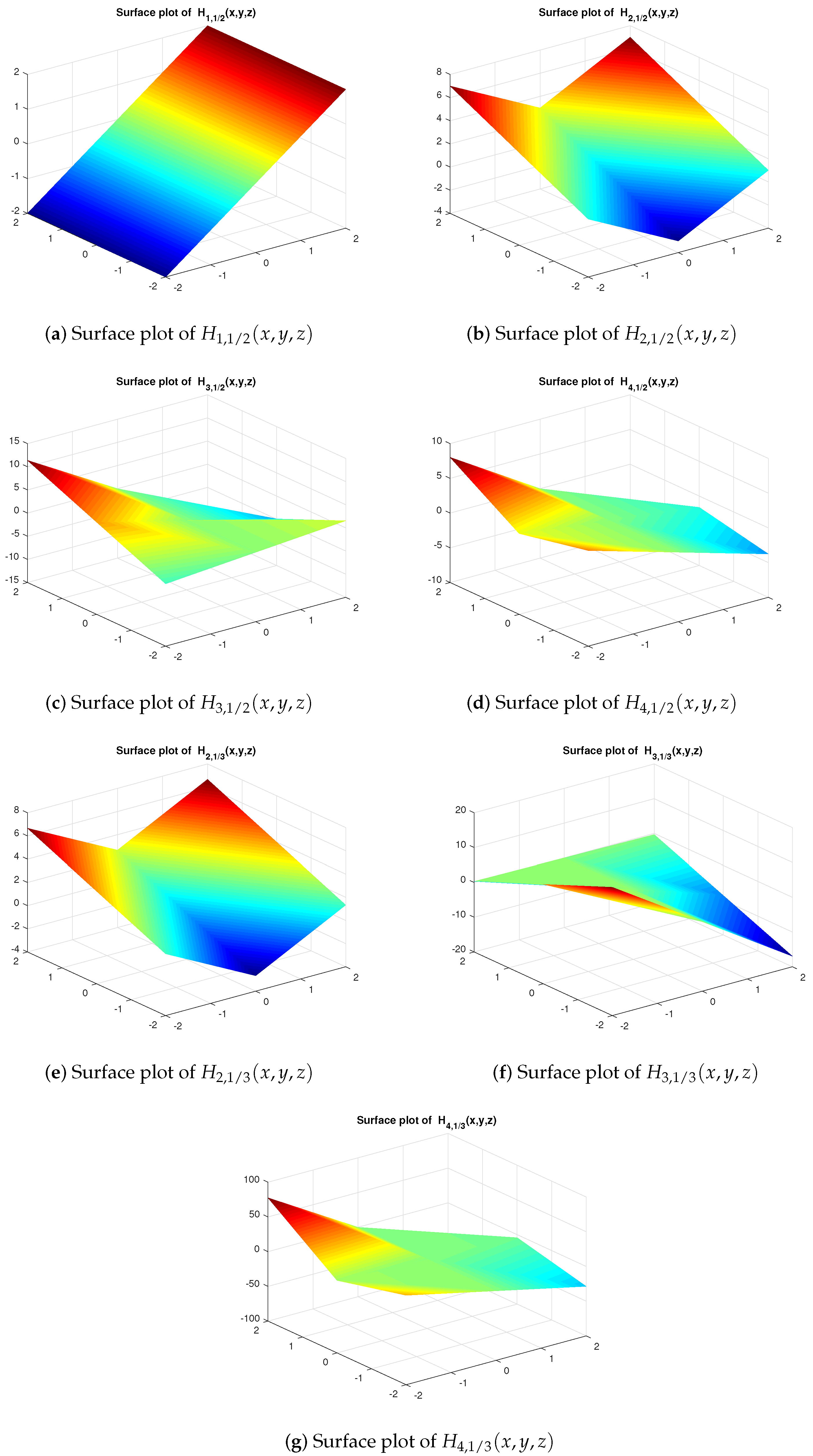
Below, some $3D$ surface diagrams of 3-variable q-Hermite polynomials $H_{n,q}(x,y,z)$ are plotted via Matlab to present their geometric appearance (see Figure 1; for $n=1,2,3,4$ and $q=\frac{1}{2},\frac{1}{3}$).

3. Auxiliary Results and Properties for 3V$\mathit{q}$HP

In this section, we will introduce some auxiliary results and characteristics for q-Hermite polynomials with three variables. Also, we establish recurrence connections and differential equations for 3VqHP $H_{n,q}(x,y,z)$.

Currently, replacing x, y and z by $x_1+x_2$, $y_1+y_2$ and $z_1+z_2$, respectively, in Equation (22) gives the following new generating functions for $H_{n,q}(x_1+x_2,y,z)$, $H_{n,q}(x,y_1+y_2,z)$ and $H_{n,q}(x,y,z_1+z_2)$:

Proposition 1.

The following new generating functions for $H_{n,q}(x_1+x_2,y,z),H_{n,q}(x,y_1+y_2,z)$ and $H_{n,q}(x,y,z_1+z_2)$ hold true:

$$e_q\left(x_{1}t\right)e_q\left(x_{2}t\right)e_q\left(y{t}^2\right)e_q\left(z{t}^3\right)=\sum _{n=0}^{\infty }{H}_{n,q}(x_1+x_2,y,z)\frac{t^n}{{\left[n\right]}_q!},$$

(30)

$$e_q\left(xt\right)e_q\left(y_{1}t\right)e_q\left(y_2{t}^2\right)e_q\left(z{t}^3\right)=\sum _{n=0}^{\infty }{H}_{n,q}(x,y_1+y_2,z)\frac{t^n}{{\left[n\right]}_q!}$$

(31)

and

$$e_q\left(xt\right)e_q\left(y{t}^2\right)e_q\left(z_1{t}^3\right)e_q\left(z_2{t}^3\right)=\sum _{n=0}^{\infty }{H}_{n,q}(x,y,z_1+z_2)\frac{t^n}{{\left[n\right]}_q!}.$$

(32)

We now establish the series expressions for $H_{n,q}(x_1+x_2,y,z),H_{n,q}(x,y_1+y_2,z)$ and $H_{n,q}(x,y,z_1+z_2)$ as follows:

Theorem 1.

The following series expressions for $H_{n,q}(x_1+x_2,y,z),H_{n,q}(x,y_1+y_2,z)$ and $H_{n,q}(x,y,z_1+z_2)$ hold true:

$$H_{n,q}(x_1+x_2,y,z)=\sum _{k=0}^n{\left[\begin{array}{c}n\\ k\end{array}\right]}_q{H}_{k,q}(x_1,y,z)x_2^{n-k},$$

(33)

$$H_{n,q}(x,y_1+y_2,z)={\left[n\right]}_q!\sum _{k=0}^{\left[n/2\right]}\frac{H_{k,q}(x,,y_1,z)y_2^{n-2k}}{{\left[k\right]}_q!{[n-2k]}_q!}$$

(34)

and

$$H_{n,q}(x,y,z_1+z_2)={\left[n\right]}_q!\sum _{k=0}^{\left[n/3\right]}\frac{H_{k,q}(x,y,z_1)z_2^{n-3k}}{{\left[k\right]}_q!{[n-3k]}_q!}.$$

(35)

Proof. 

Dilating the left-hand aspect of Equation (30) by utilizing Equation (15), we obtain

$$\sum _{n=0}^{\infty }{x}_2^n\frac{t^n}{{\left[n\right]}_q!}\sum _{k=0}^{\infty }{H}_{k,q}(x_1,y,z)\frac{t^k}{{\left[k\right]}_q!}=\sum _{n=0}^{\infty }{H}_{n,q}(x_1+x_2,y,z)\frac{t^n}{{\left[n\right]}_q!}.$$

By examining the corresponding powers of t on each aspect of the above equation and using Equation (14),we obtain claim (33).

Similar to obtaining the series expression (33), by utilizing Equation (15) to expand the left-hand aspect of Equations (31) and (32), correspondingly, and then using the identical procedures applied to prove Equation (33), we obtain the claims (34) and (35). The proof of Theorem 1 is completed. □

From Equation (33), we deduce the following result immediately:

Corollary 1.

The following series expressions for $H_{n,q}(x_1+x_2,y_1+y_2,z)$ and $H_{n,q}(x_1+x_2,y_1+y_2,z_1+z_2)$ hold true:

$$H_{n,q}(x_1+x_2,y_1+y_2,z)=\sum _{k=0}^n{\left[\begin{array}{c}n\\ k\end{array}\right]}_q{H}_{k,q}(x_1,y_1,z_1)H_{n-k,q}(x_2,y_2)$$

(36)

and

$$H_{n,q}(x_1+x_2,y_1+y_2,z_1+z_2)=\sum _{k=0}^n{\left[\begin{array}{c}n\\ k\end{array}\right]}_q{H}_{k,q}(x_1,y_1,z_1)H_{n-k,q}(x_2,y_2,z_2).$$

(37)

Remark 2.

Formula (25) makes it easy to verify that

$$H_{n,q}(ax,a^{2}y,a^{3}z)=a^n{H}_{n,q}(x,y,z),$$

(38)

in which a is a fixed value.

The subsequent theorem is used to prove the q-partial derivatives for 3VqHP $H_{n,q}(x,y,z)$:

Theorem 2.

The following q-partial derivatives for $H_{n,q}(x,y,z)$ hold true:

$$D_{q,x}{H}_{n,q}(x,y,z)={\left[n\right]}_q{H}_{n-1,q}(x,y,z),n\ge 1,$$

(39)

$$D_{q,y}\left(H_{n,q}(x,y,z)\right)={\left[n\right]}_q{[n-1]}_q{H}_{n-2,q}(x,y,z),n\ge 2,$$

(40)

$$D_{q,z}{H}_{n,q}(x,y,z)={\left[n\right]}_q{[n-1]}_q{[n-2]}_q{H}_{n-3,q}(x,y,z),n\ge 3,$$

(41)

$$D_{q,x}^m\left(H_{n,q}(x,y,z)\right)=\frac{{\left[n\right]}_q!}{{[n-m]}_q!}{H}_{n-m,q}(x,y,z),0\le m\le n,$$

(42)

$$D_{q,y}^m\left(H_{n,q}(x,y,z)\right)=\frac{{\left[n\right]}_q!}{{[n-2m]}_q!}{H}_{n-2m,q}(x,y,z),0\le m\le \frac{n}{2}$$

(43)

and

$$D_{q,z}^m\left(H_{n,q}(x,y,z)\right)=\frac{{\left[n\right]}_q!}{{[n-3m]}_q!}{H}_{n-3m,q}(x,y,z),0\le m\le \frac{n}{3}.$$

(44)

Proof. 

Applying the q-partial derivative of each aspect of Equation (22) with regard to x and plugging it into Equation (19) for $m=1$, we receive

$$t{e}_q\left(xt\right)e_q\left(y{t}^2\right)e_q\left(z{t}^3\right)=\sum _{n=0}^{\infty }{D}_{q,x}{H}_{n,q}(x,y,z)\frac{t^n}{{\left[n\right]}_q!}.$$

Applying Equation (22) on the left part of Equation (3) provides us

$$\sum _{n=1}^{\infty }{H}_{n-1,q}(x,y,z)\frac{t^n}{{[n-1]}_q!}=\sum _{n=0}^{\infty }{D}_{q,x}{H}_{n,q}(x,y,z)\frac{t^n}{{\left[n\right]}_q!}.$$

Therefore, when the corresponding values of t from each aspect are compared, we obtain assertion (39).

After that, we take the q-partial derivative of each aspect of Equation (22) with regard to y and z and then repeat the procedures in the equation’s proof (39), to obtain assertions (40) and (41), respectively.

Once more, using the techniques from obtaining Equation (39), we take the 2^nd order q-partial derivative for two aspects of Equation (22) with regard to x, then utilizing Equation (19), we obtain

$$D_{q,x}^2{H}_{n,q}(x,y,z)={\left[n\right]}_q{[n-1]}_q{H}_{n-2,q}(x,y,z),n\ge 2.$$

(45)

Likewise, taking the $m^{th}$ degree q-partial derivative of each aspect of Equation (22) with regard to x, then via Equation (19) and repeating the previous steps of proving Equation (39), we obtain assertion (42).

In the same way, if we take the $m^{th}$ order q-partial derivatives of each aspect of Equation (22) with regard to y and z, then continue the exact same procedure, we receive assertions (43) and (44). The proof of Theorem 2 is completed. □

Once more, for $m=2,3$ in Equation (42) and utilizing Equations (40), (41) and (45), we obtain the subsequent q-partial differential equations for 3VqHP $H_{n,q}(x,y,z)$:

Corollary 2.

The q-partial differential equations for 3VqHP $H_{n,q}(x,y,z)$ are listed below:

$$D_{q,x}^2{H}_{n,q}(x,y,z)=D_{q,y}{H}_{n,q}(x,y,z)$$

(46)

and

$$D_{q,x}^3{H}_{n,q}(x,y,z)=D_{q,z}{H}_{n,q}(x,y,z).$$

(47)

Following that, we set up the recurrence relations for 3VqHP $H_{n,q}(x,y,z)$. To accomplish this, we have to show the subsequent lemma:

Lemma 1.

The q-partial derivative of $e_q\left(z{t}^3\right)$ with regard to t can be expressed by the following recurrence relation:

$$D_{q,t}{e}_q\left(z{t}^3\right)=z{t}^2{e}_q\left(z{t}^3\right)+qz{t}^2{e}_q\left(qz{t}^3\right)+q^{2}z{t}^2{e}_q\left(q^{2}z{t}^3\right),$$

(48)

where the operator $D_{q,t}$ is defined as Formula (2).

Proof. 

By (18) and (15), we obtain

$$D_{q,t}{e}_q\left(z{t}^3\right)=\sum _{n=0}^{\infty }\frac{z^n{\left[3n\right]}_q{t}^{3-1}}{{\left[n\right]}_q!}.$$

(49)

Using (13), we obtain

$$\frac{{\left[3n\right]}_q}{{\left[n\right]}_q}=1+q^n+q^{2n}.$$

(50)

Hence, combining (49) and (50) gives

$$\begin{array}{cc}\hfill D_{q,t}{e}_q\left(z{t}^3\right)& =\sum _{n=1}^{\infty }\frac{z^n(1+q^n+q^{2n})t^{3n-1}}{{[n-1]}_q!}\hfill \\ \hfill & =\sum _{n=0}^{\infty }\frac{z^{n+1}{t}^{3n+2}}{{\left[n\right]}_q!}+\sum _{n=0}^{\infty }\frac{{\left(qz\right)}^{n+1}{t}^{3n+2}}{{\left[n\right]}_q!}+\sum _{n=0}^{\infty }\frac{{\left(q^{2}z\right)}^{n+1}{t}^{3n+2}}{{\left[n\right]}_q!}\hfill \\ \hfill & =z{t}^2\sum _{n=0}^{\infty }\frac{{\left(z{t}^3\right)}^n}{{\left[n\right]}_q!}+qz{t}^2\sum _{n=0}^{\infty }\frac{{\left(qz{t}^3\right)}^n}{{\left[n\right]}_q!}+q^{2}z{t}^2\sum _{n=0}^{\infty }\frac{{\left(q^{2}z{t}^3\right)}^n}{{\left[n\right]}_q!},\hfill \end{array}$$

which can be easily simplified as (48) by virtue of Formula (15). The proof of Lemma 1 is completed. □

Remark 3.

It is easy to see that for $q\to 1^{-}$, we have $D_{q,t}$→$D_t$ and $e_q\left(z{t}^3\right)$→$e^{z{t}^3}$. So, by applying Lemma 1 with $q\to 1^{-}$, we can obtain the commonly used ordinary calculus result:

$$D_t{e}^{z{t}^3}=3z{t}^2{e}^{z{t}^3},$$

where $D_t$ represents the t-dependent ordinary derivative.

The subsequent theorem is used to prove the existence of the pure recurrence relation for the 3VqHP $H_{n,q}(x,y,z)$:

Theorem 3.

For $n\ge 2$, the recurrence relation for 3-variable q-Hermite polynomials $H_{n,q}(x,y,z)$ can be represented by

$$\begin{array}{c}\hfill H_{n+1,q}(x,y,z)=x{H}_{n,q}(x,qy,qz)+y{\left[n\right]}_q\left(H_{n-1,q}(x,y,qz)+q{H}_{n-1,q}(x,qy,qz)\right)\\ \hfill +z{\left[n\right]}_q{[n-1]}_q\left(H_{n-2,q}(x,y,z)+q{H}_{n-2,q}(x,y,qz)+q^2{H}_{n-2,q}(x,y,q^{2}z)\right).\end{array}$$

(51)

Proof. 

By virtue of Formula (20) for q-differentiation and with the help of the q-derivative of the two aspects of Equation (22) with regard to t, we can easily acquire

$${\sum }_{n=0}^{\infty }{D}_{q,t}{H}_{n,q}(x,y,z)\frac{t^n}{{\left[n\right]}_q!}=\left[D_{q,t}{e}_q\left(xt\right)e_q\left(qy{t}^2\right)+e_q\left(xt\right)D_{q,t}(e_q\left(y{t}^2\right)\right]e_q\left(qz{t}^3\right)+\left[e_q\left(xt\right)e_q\left(y{t}^2\right)\right]D_{q,t}{e}_q\left(z{t}^3\right).$$

(52)

Using Equations (21) and (48) in the right aspect part of (52) and Formula (18) in the left aspect part of (52), respectively, we obtain

$$\begin{array}{cc}{\sum }_{n=1}^{\infty }{H}_{n,q}(x,y,z)\frac{t^{n-1}}{{[n-1]}_q!}\hfill & =x{e}_q\left(xt\right)e_q\left(qy{t}^2\right)e_q\left(qz{t}^3\right)+yt{e}_q\left(xt\right)e_q\left(y{t}^2\right)e_q\left(qz{t}^3\right)+qyt{e}_q\left(xt\right)e_q\left(qy{t}^2\right)e_q\left(qz{t}^3\right)\hfill \\ & +z{t}^2{e}_q\left(xt\right)e_q\left(y{t}^2\right)e_q\left(z{t}^3\right)+qz{t}^2{e}_q\left(xt\right)e_q\left(y{t}^2\right)e_q\left(qz{t}^3\right)+q^{2}z{t}^2{e}_q\left(xt\right)e_q\left(y{t}^2\right)e_q\left(q^{2}z{t}^3\right).\hfill \end{array}$$

(53)

Finally, utilizing Equation (22) on the left part of (53) and contrasting the two corresponding powers of t on both parts of the outcome equation, we can derive our claim (51). The proof of Theorem 3 is completed. □

Example 1.

Applying Formula (51), we have the following:

$$\begin{array}{c}{H}_{3,2/3}(x,y,z)=x{H}_{2,2/3}\left(x,\frac{2}{3}y,\frac{2}{3}z\right)+\frac{5}{3}y\left(H_{1,2/3}\left(x,y,\frac{2}{3}z\right)+\frac{2}{3}{H}_{1,2/3}\left(x,\frac{2}{3}y,\frac{2}{3}z\right)\right)\hfill \\ \hfill +\frac{5}{3}z\left(H_{0,2/3}(x,y,z)+\frac{2}{3}{H}_{0,2/3}\left(x,y,\frac{2}{3}z\right)+\frac{4}{9}{H}_{0,2/3}\left(x,y,\frac{4}{9}z\right)\right),\end{array}$$

$$\begin{array}{c}{H}_{4,2/3}(x,y,z)=x{H}_{3,2/3}\left(x,\frac{2}{3}y,\frac{2}{3}z\right)+\frac{19}{9}y\left(H_{2,2/3}\left(x,y,\frac{2}{3}z\right)+\frac{2}{3}{H}_{2,2/3}\left(x,\frac{2}{3}y,\frac{2}{3}z\right)\right)\hfill \\ \hfill +\frac{1185}{243}z\left(H_{1,2/3}(x,y,z)+\frac{2}{3}{H}_{1,2/3}\left(x,y,\frac{2}{3}z\right)+\frac{4}{9}{H}_{1,2/3}\left(x,y,\frac{4}{9}z\right)\right),\end{array}$$

and

$$\begin{array}{c}{H}_{5,2/3}(x,y,z)=x{H}_{4,2/3}\left(x,\frac{2}{3}y,\frac{2}{3}z\right)+\frac{65}{27}y\left(H_{3,2/3}\left(x,y,\frac{2}{3}z\right)+\frac{2}{3}{H}_{3,2/3}\left(x,\frac{2}{3}y,\frac{2}{3}z\right)\right)\hfill \\ \hfill +\frac{13715}{2187}z\left(H_{2,2/3}(x,y,z)+\frac{2}{3}{H}_{2,2/3}\left(x,y,\frac{2}{3}z\right)+\frac{4}{9}{H}_{2,2/3}\left(x,y,\frac{4}{9}z\right)\right).\end{array}$$

The following theorem is very important and will be used to prove the existence of a q-differential recurrence relation for 3-variable q-Hermite polynomials $H_{n,q}(x,y,z)$.

Theorem 4.

The q-differential recurrence relation for 3-variable q-Hermite polynomials $H_{n,q}(x,y,z)$ can be represented by

$$\begin{array}{c}{\left[n\right]}_q{H}_{n,q}(x,y,z)=x{D}_{q,x}{H}_{n,q}(x,qy,qz)+y{D}_{q,x}^2\left(H_{n,q}(x,y,qz)+q{H}_{n,q}(x,qy,qz)\right)\\ +z{\left[n\right]}_q{D}_{q,x}^2\left(H_{n-1,q}(x,y,z)+q{H}_{n-1,q}(x,y,qz)+q^2{H}_{n-1,q}(x,y,q^{2}z)\right),\end{array}$$

(54)

or, equivalently

$$\begin{array}{c}{\left[n\right]}_q{H}_{n,q}(x,y,z)=x{D}_{q,x}{H}_{n,q}(x,qy,qz)+y{D}_{q,y}\left(H_{n,q}(x,y,qz)+q{H}_{n,q}(x,qy,qz)\right)\\ +z{\left[n\right]}_q{D}_{q,y}\left(H_{n-1,q}(x,y,z)+q{H}_{n-1,q}(x,y,qz)+q^2{H}_{n-1,q}(x,y,q^{2}z)\right).\end{array}$$

(55)

Proof. 

From Equation (38), we obtain

$$H_{n-1,q}(x,y,qz)=q^{n-1}{H}_{n-1,q}\left(\frac{1}{q}x,\frac{1}{q^2}y,\frac{1}{q^2}z\right),$$

which, when applied to Equation (39), gives

$$H_{n-1,q}(x,y,qz)=\frac{q^n}{{\left[n\right]}_q}{D}_{q,x}{H}_{n,q}\left(\frac{1}{q}x,\frac{1}{q^2}y,\frac{1}{q^2}z\right).$$

(56)

Further, by plugging Equation (38) into the right aspect of Equation (56), we have

$$H_{n-1,q}(x,y,qz)=\frac{1}{{\left[n\right]}_q}{D}_{q,x}{H}_{n,q}\left(x,y,qz\right).$$

(57)

Similarly, by following the same methods involved in obtaining Equation (57), we have

$$H_{n-1,q}(x,qy,qz)=\frac{1}{{\left[n\right]}_q}{D}_{q,x}{H}_{n,q}\left(x,qy,qz\right).$$

(58)

From Equation (38), we achieve

$$H_{n-2,q}(x,y,q^{2}z)=q^{n-2}{H}_{n-2,q}\left(\frac{1}{q}x,\frac{1}{q^2}y,\frac{1}{q}z\right).$$

By plugging in Equation (40) or (42), we attain

$$H_{n-2,q}(x,y,q^{2}z)=\frac{q^n}{{\left[n\right]}_q{[n-1]}_q}{D}_{q,y}{H}_{n,q}\left(\frac{1}{q}x,\frac{1}{q^2}y,\frac{1}{q^2}z\right),$$

(59)

or, equivalently

$$H_{n-2,q}(x,y,q^{2}z)=\frac{q^n}{{\left[n\right]}_q{[n-1]}_q}{D}_{q,x}^2{H}_{n,q}\left(\frac{1}{q}x,\frac{1}{q^2}y,\frac{1}{q}z\right).$$

(60)

Once again, utilizing Equation (38) on the right aspect of Equations (59) and (60), we have

$$H_{n-2,q}(x,y,q^{2}z)=\frac{1}{{\left[n\right]}_q{[n-1]}_q}{D}_{q,y}{H}_{n,q}\left(x,y,q^{2}z\right),$$

(61)

or, equivalently

$$H_{n-2,q}(x,y,q^{2}z)=\frac{1}{{\left[n\right]}_q{[n-1]}_q}{D}_{q,x}^2{H}_{n,q}\left(x,y,q^{2}z\right).$$

(62)

Similarly, by following the same methods involved in obtaining Equation (62), we attain

$$H_{n-2,q}(x,y,qz)=\frac{1}{{\left[n\right]}_q{[n-1]}_q}{D}_{q,y}{H}_{n,q}\left(x,y,qz\right),$$

(63)

or, equivalently

$$H_{n-2,q}(x,y,qz)=\frac{1}{{\left[n\right]}_q{[n-1]}_q}{D}_{q,x}^2{H}_{n,q}\left(x,y,qz\right).$$

(64)

Using Equations (57), (62) and (64) or (63) in the right aspect of Equation (51), we prove Formulas (54) or (55). The proof of Theorem 4 is completed. □

Applying Theorem 4, we can establish the following new q-differential recurrence relations for 3-variable q-Hermite polynomials $H_{n,q}(x,y,z)$:

Theorem 5.

The q-differential recurrence relation for 3-variable q-Hermite polynomials $H_{n,q}(x,y,z)$ can be represented by

$$\begin{array}{c}{H}_{n+1,q}(x,y,z)=x{H}_{n,q}(x,qy,qz)+y{D}_{q,x}\left(H_{n,q}(x,y,qz)+q{H}_{n,q}(x,qy,qz)\right)\\ +z{D}_{q,x}^2\left(H_{n,q}(x,y,z)+q{H}_{n,q}(x,y,qz)+q^2{H}_{n,q}(x,y,q^{2}z))\right),\end{array}$$

(65)

or, equivalently

$$\begin{array}{c}{H}_{n+1,q}(x,y,z)=x{H}_{n,q}(x,qy,qz)+y{D}_{q,x}\left(H_{n,q}(x,y,qz)+q{H}_{n,q}(x,qy,qz)\right)\\ +z{D}_{q,y}\left(H_{n,q}(x,y,z)+q{H}_{n,q}(x,y,qz)+q^2{H}_{n,q}(x,y,q^{2}z))\right).\end{array}$$

(66)

Proof. 

Changing n in Equation (51) to $n-1$ yields

$$\begin{array}{c}{H}_{n,q}(x,y,z)=x{H}_{n-1,q}(x,qy,qz)+y{[n-1]}_q\left(H_{n-2,q}(x,y,qz)+q{H}_{n-2,q}(x,qy,qz)\right)\\ +z{[n-1]}_q{[n-2]}_q\left(H_{n-3,q}(x,y,z)+q{H}_{n-3,q}(x,y,qz)+q^2{H}_{n-3,q}(x,y,q^{2}z))\right),n\ge 3.\end{array}$$

(67)

As with direct steps involved in obtaining (54) or (55), we obtain Formulas (65) or (66). The proof of Theorem 5 is completed. □

In order to establish the differential equation of the q-Hermite polynomials of three variables $H_{n,q}(x,y,z)$, we define the concept of shift operators as follows:

Definition 2.

The shift operators $L_{a,x}$, $L_{a,y}$ and $L_{a,z},$ which are employed whenever $f(x,y,z)$ represents a q-function via three variables, are described as follows:

$$L_{a,x}f(x,y,z)=f(ax,y,z),$$

(68)

$$L_{a,y}f(x,y,z)=f(x,ay,z)$$

(69)

and

$$L_{a,z}f(x,y,z)=f(x,y,az),$$

(70)

where a represents a constant.

Remark 4.

(a) 

It is worth mentioning that Formula (68) shows that the shift operator $L_{a,x}$ has the subsequent characteristics:

$$L_{a,x}{L}_{b,x}{L}_{c,x}f(x,y,z)=f(abcx,y,z)=L_{abc,x}f(x,y,z).$$

(71)

(b) 

Specifically, for the case a = b = c, we have

$$L_{a^3,x}f(x,y,z)=f(a^{3}x,y,z)=L_{a,x}{L}_{a,x}{L}_{a,x}f(x,y,z)=L_{a,x}^{3}f(x,y,z).$$

(72)

(c) 

If $L_{a,x}^{-1}$ is the opposite of the expression $L_{a,x}$, then $L_{a,x}^{-1}{L}_{a,x}=I$, where I is an identity operator, which is so $If(x,y,z)=f(x,y,z).$ In accordance with Equation (68), we have

$$L_{a,x}^{-1}f(ax,y,z)=f(x,y,z).$$

Presently, we demonstrate the next result for a q-differential equation of 3-variable q-Hermite polynomials $H_{n,q}(x,y,z)$ by using shift operators:

Theorem 6.

The 3-variable q-Hermite polynomials $H_{n,q}(x,y,z)$ comply with the subsequent q-differential equation:

$$\begin{array}{c}\hfill \left[z(1+q{L}_{q,z}+q^2{L}_{q,z})D_{q,x}^3+y(L_{q,z}+q{L}_{q,z})D_{q,x}^2+x{L}_{q,x,y}{D}_{q,x}-{\left[n\right]}_q\right]H_{n,q}(x,y,z)=0,\end{array}$$

(73)

where $L_{q,x,y}:=L_{q,x}{L}_{q,y}$ (see [31]).

Proof. 

Following a similar argument as in the proof of (64), we obtain

$$H_{n-3,q}(x,y,qz)=\frac{1}{{\left[n\right]}_q{[n-1]}_q{[n-2]}_q}{D}_{q,x}^3{H}_{n,q}\left(x,y,qz\right).$$

(74)

Also, in the same procedure it is obvious to obtain

$$H_{n-3,q}(x,y,q^{2}z)=\frac{1}{{\left[n\right]}_q{[n-1]}_q{[n-2]}_q}{D}_{q,x}^3{H}_{n,q}(x,y,q^{2}z).$$

(75)

Using Equations (58), (64), (74) and (75) on the right aspect of the Formula (67), we obtain

$$\begin{array}{cc}\hfill H_{n,q}(x,y,z)& =x\frac{1}{{\left[n\right]}_q}{D}_{q,x}{H}_{n,q}(x,qy,qz)+y{[n-1]}_q(\frac{1}{{\left[n\right]}_q{[n-1]}_q}{D}_{q,x}^2{H}_{n,q}(x,y,qz)\hfill \\ \hfill & +q\frac{1}{{\left[n\right]}_q{[n-1]}_q}{D}_{q,x}^2{H}_{n,q}(x,qy,qz))+{[n-1]}_q{[n-2]}_{q}z(\frac{1}{{\left[n\right]}_q{[n-1]}_q{[n-2]}_q}{D}_{q,x}^3{H}_{n,q}\left(x,y,z\right)\hfill \\ \hfill & +q\frac{1}{{\left[n\right]}_q{[n-1]}_q{[n-2]}_q}{D}_{q,x}^3{H}_{n,q}\left(x,y,qz\right)+q^2\frac{1}{{\left[n\right]}_q{[n-1]}_q{[n-2]}_q}{D}_{q,x}^3{H}_{n,q}\left(x,y,q^{2}z\right)),\hfill \end{array}$$

which on simplification and using Equation (68) gives claim (73). The proof of Theorem 6 is completed. □

Example 2.

Applying Formula (73), we obtain the following:

$$\left[z\left(1+\frac{2}{3}{L}_{2/3,z}+\frac{4}{9}{L}_{2/3,z}\right)D_{2/3,x}^3+y\left(L_{2/3,z}+\frac{2}{3}{L}_{2/3,z}\right)D_{2/3,x}^2+x{L}_{2/3,x,y}{D}_{2/3,x}-1\right]H_{1,2/3}(x,y,z)=0,$$

$$\left[z\left(1+\frac{4}{5}{L}_{4/5,z}+\frac{16}{25}{L}_{4/5,z}\right)D_{4/5,x}^3+y\left(L_{4/5,z}+\frac{4}{5}{L}_{4/5,z}\right)D_{4/5,x}^2+x{L}_{4/5,x,y}{D}_{4/5,x}-\frac{9}{4}\right]H_{2,4/5}(x,y,z)=0,$$

and

$$\left[z\left(1+\frac{5}{6}{L}_{5/6,z}+\frac{25}{36}{L}_{5/6,z}\right)D_{5/6,x}^3+y\left(L_{5/6,z}+\frac{5}{6}{L}_{5/6,z}\right)D_{5/6,x}^2+x{L}_{5/6,x,y}{D}_{q,x}-\frac{91}{36}\right]H_{3,5/6}(x,y,z)=0.$$

Remark 5.

For $q\to 1^{-}$, Equations (22) and (25) reduce to Equations (1) and (2) for $H_n(x,y,z)$. Also, for $q\to 1^{-}$, Equations (39)–(48) reduce to the respective results for $H_n(x,y,z)$ given by Equations (3)–(8). Further, for $q\to 1^{-}$, Equations (51), (54) or (55) and (65) or (66) give the differential recurrence relations for 3-variable Hermite polynomials $H_n(x,y,z)$. Finally, for $q\to 1^{-}$, Equation (73) reduces to Equation (9).

4. Operational and Summation Formulas

In this section, we create operational and summation formulas for 3-variable q-Hermite polynomials $H_{n,q}(x,y,z)$ as well as their various q-derivatives. We now demonstrate the following.

Theorem 7.

The 3-variable q-Hermite polynomials $H_{n,q}(x,y,z)$ satisfy the following operational identity

$$H_{n,q}(x,y,z)=e_q\left(y{D}_{q,x}^2\right)e_q\left(z{D}_{q,x}^3\right)x^n,$$

(76)

where $D_{q,x}^2$ and $D_{q,x}^3$ are the second and third q-derivative operators.

Proof. 

It is possible to check if the following feature is true for the q-differential operator $D_{q,x}$:

$$D_{q,x}^r{x}^n=\frac{{\left[n\right]}_q!}{{[n-r]}_q!}{x}^{n-r}.$$

(77)

From Equation (77), we obtain

$$D_{q,x}^{3r}{H}_{n,q}(x,y)=\frac{{\left[n\right]}_q!}{{[n-3r]}_q!}{H}_{n-3r,q}(x,y).$$

(78)

Putting the previous equation into the right part of Equation (25), we attain

$$H_{n,q}(x,y,z)=\sum _{r=0}^{\infty }\frac{{\left(z{D}_{q,x}^3\right)}^r{H}_{n,q}(x,y)}{{\left[r\right]}_q!}.$$

Utilizing Equation (15) on the right part of the preceding formula provides

$$H_{n,q}(x,y,z)=e_q\left(z{D}_{q,x}^3\right)H_{n,q}(x,y).$$

Therefore, using expression (12) on the right side of the preceding equation yields Formula (76). The proof is completed. □

In the structure of the subsequent statement, we cultivate summation formulas for the q-Hermite polynomials with three variables $H_{n,q}(x,y,z)$ in the structure of the subsequent statement:

Theorem 8.

The 3-variable q-Hermite polynomials $H_{n,q}(x,y,z)$ fulfill the subsequent summing formulas:

$${\left[n\right]}_q!\sum _{r=0}^{\left[n/3\right]}\frac{H_{n-3r,q}(x,y,z)q^{{(}_2^r)}{(-z)}^r}{{[n-3r]}_q!{\left[r\right]}_q!}=H_{n,q}(x,y).$$

(79)

In particular, we have the following:

(a) 

If $n=3m$ ($m\in \mathbb{N}$), then

$${\left[3m\right]}_q!\sum _{r=0}^{\left[3m/2\right]}\frac{q^{{(}_2^r)}{(-y)}^r{H}_{3m-2r,q}(x,y,z)}{{\left[r\right]}_q!{[3m-2r]}_q!}=H_{3m,q}(x,z).$$

(80)

(b) 

If $n=3m+1$ ($m\in \mathbb{N}\cup \left\{0\right\}$), then

$${[3m+1]}_q!\sum _{r=0}^{\left[3m+1/2\right]}\frac{q^{{(}_2^r)}{(-y)}^r{H}_{3m+1-2r,q}(x,y)}{{\left[r\right]}_q!{[3m+1-2r]}_q!}=0.$$

(81)

Proof. 

In the context of Equation (17), it is clear

$$e_q\left(xt\right)e_q\left(y{t}^2\right)e_q\left(z{t}^3\right)E_q(-z{t}^3)=e_q\left(xt\right)e_q\left(y{t}^2\right),$$

(82)

which, on using Equations (10), (16) and (22), gives

$$\sum _{n=0}^{\infty }\sum _{r=0}^{\infty }\frac{H_{n,q}(x,y,z)q^{{(}_2^r)}{(-z)}^r{t}^{n+3r}}{{\left[n\right]}_q!{\left[r\right]}_q!}=\sum _{n=0}^{\infty }{H}_{n,q}(x,y)\frac{t^n}{{\left[n\right]}_q!}.$$

Utilizing Formula (24) in the left aspect of the previous equation, we obtain

$$\sum _{n=0}^{\infty }\sum _{r=0}^{\left[n/3\right]}\frac{H_{n-3r,q}(x,y,z)q^{{(}_2^r)}{(-z)}^r{t}^n}{{[n-3r]}_q!{\left[r\right]}_q!}=\sum _{n=0}^{\infty }{H}_{n,q}(x,y)\frac{t^n}{{\left[n\right]}_q!},$$

Comparing the identical powers of t on each side gives rise to statement (79). Using Equation (17) once more, we obtain

$$E_q(-y{t}^2)e_q\left(xt\right)e_q\left(y{t}^2\right)e_q\left(z{t}^3\right)=e_q\left(xt\right)e_q\left(z{t}^3\right).$$

(83)

Putting (16) and (22) into the aforementioned equation provides us

$$\sum _{n=0}^{\infty }\sum _{r=0}^{\infty }\frac{q^{{(}_2^r)}{(-y)}^r{H}_{n,q}(x,y,z)t^{n+2r}}{{\left[n\right]}_q!{\left[r\right]}_q!}=\sum _{n=0}^{\infty }{H}_{n,q}^{\left(3\right)}(x,z)\frac{t^n}{{\left[n\right]}_q!},$$

This, when applied to Equation (23), yields

$$\sum _{n=0}^{\infty }\sum _{r=0}^{\left[n/2\right]}\frac{q^{{(}_2^r)}{(-y)}^r{H}_{n-2r,q}(x,y,z)t^n}{{\left[r\right]}_q!{[n-2r]}_q!}=\sum _{n=0}^{\infty }{H}_{n,q}^{\left(3\right)}(x,z)\frac{t^n}{{\left[n\right]}_q!}.$$

(84)

When each of the even as well as odd values of t from each side of Equation (84) are compared, we obtain statements (80) and (81). The proof is completed. □

Remark 6.

It is worth to mentioning that the corresponding expression of the summation formula, provided in Equation (81), is as outlined below:

$$\sum _{r=0}^{\left[3m/2\right]}\frac{q^{{(}_2^r)}{(-y)}^r{H}_{3m-2r,q}(x,y,z)}{{\left[r\right]}_q!{[3m-2r]}_q!}=\frac{q^{\left(\genfrac{}{}{0pt}{}{\frac{3m+1}{2}}{2}\right)}{y}^{\frac{3m+1}{2}}}{{\left[\frac{3m+1}{2}\right]}_q!}.$$

(85)

By using Equation (39) in Theorem 8 and Remark 6, we drive the following summation formulas for the q-derivative of $H_{n,q}(x,y,z)$ with regard to x.

Corollary 3.

The subsequent summation formulas are valid:

$${\left[n\right]}_q!\sum _{r=0}^{\left[n/3\right]}\frac{D_{q,x}{H}_{n+1-3r,q}(x,y,z)q^{{(}_2^r)}{(-z)}^r}{{[n+1-3r]}_q!{\left[r\right]}_q!}=H_{n,q}(x,y),$$

(86)

$${\left[3m\right]}_q!\sum _{r=0}^{\left[3m/2\right]}\frac{q^{{(}_2^r)}{(-y)}^r{D}_{q,x}{H}_{3m+1-2r,q}(x,y,z)}{{\left[r\right]}_q!{[3m+1-2r]}_q!}=H_{3m,q}(x,z)$$

(87)

and

$$\sum _{r=0}^{\left[(3m+1)/2\right]}\frac{q^{{(}_2^r)}{(-y)}^r{D}_{q,x}{H}_{3m+2-2r,q}(x,y,z)}{{\left[r\right]}_q!{[3m+2-2r]}_q!}=\frac{q^{\left(\genfrac{}{}{0pt}{}{\frac{3m+1}{2}}{2}\right)}{y}^{\frac{3m+1}{2}}}{{\left[\frac{3m+1}{2}\right]}_q!}.$$

(88)

Similarly, using Equation (40) in Equations (79), (80) and (85), we acquire the subsequent summing formulas for the q-derivative of $H_{n,q}(x,y,z)$ with regard to y:

Corollary 4.

The subsequent summation formulas are valid:

$${\left[n\right]}_q!\sum _{r=0}^{\left[n/3\right]}\frac{D_{q,y}{H}_{n+2-3r,q}(x,y,z)q^{{(}_2^r)}{(-z)}^r}{{[n+2-3r]}_q!{\left[r\right]}_q!}=H_{n,q}(x,y),$$

(89)

$${\left[3m\right]}_q!\sum _{r=0}^{\left[3m/2\right]}\frac{q^{{(}_2^r)}{(-y)}^r{D}_{q,y}{H}_{3m+2-2r,q}(x,y,z)}{{\left[r\right]}_q!{[3m+2-2r]}_q!}=H_{3m,q}(x,z),$$

(90)

and

$$\sum _{r=0}^{\left[(3m+1)/2\right]}\frac{q^{{(}_2^r)}{(-y)}^r{D}_{q,y}{H}_{3m+2-2r,q}(x,y,z)}{{\left[r\right]}_q!{[3m+2-2r]}_q!}=\frac{q^{\left(\genfrac{}{}{0pt}{}{\frac{3m+1}{2}}{2}\right)}{y}^{\frac{3m+1}{2}}}{{\left[\frac{3m+1}{2}\right]}_q!}.$$

(91)

Furthermore, using Equation (41) in Equations (79), (80) and (85), we acquire the subsequent summing formulas for $H_{n,q}(x,y,z)$ with regard to z:

Corollary 5.

The subsequent summation formulas are valid:

$${\left[n\right]}_q!\sum _{r=0}^{\left[n/3\right]}\frac{D_{q,z}{H}_{n+3-3r,q}(x,y,z)q^{{(}_2^r)}{(-z)}^r}{{[n+3-3r]}_q!{\left[r\right]}_q!}=H_{n,q}(x,y),$$

(92)

$${\left[3m\right]}_q!\sum _{r=0}^{\left[3m/2\right]}\frac{q^{{(}_2^r)}{(-y)}^r{D}_{q,z}{H}_{3m+3-2r,q}(x,y,z)}{{\left[r\right]}_q!{[3m+3-2r]}_q!}=H_{3m,q}(x,z),$$

(93)

and

$$\sum _{r=0}^{\left[(3m+1)/2\right]}\frac{q^{{(}_2^r)}{(-y)}^r{D}_{q,z}{H}_{3m+3-2r,q}(x,y,z)}{{\left[r\right]}_q!{[3m+3-2r]}_q!}=\frac{q^{\left(\genfrac{}{}{0pt}{}{\frac{3m+1}{2}}{2}\right)}{y}^{\frac{3m+1}{2}}}{{\left[\frac{3m+1}{2}\right]}_q!}.$$

(94)

Example 3.

Applying Formulas (79), (86), (89) and (92), we obtain the following:

$$\begin{array}{c}{H}_{7,2/3}(x,y,z)-{\left[7\right]}_{2/3}{\left[6\right]}_{2/3}{\left[5\right]}_{2/3}z{H}_{4,2/3}(x,y,z)\\ +{\left[7\right]}_{2/3}{\left[6\right]}_{2/3}{\left[5\right]}_{2/3}{\left[4\right]}_{2/3}{\left[3\right]}_{2/3}{z}^2{H}_{1,2/3}(x,y,z)(2/3)=H_{7,2/3}(x,y),\end{array}$$

(95)

$$\frac{1}{{\left[4\right]}_{4/5}}{D}_{4/5,x}{H}_{3,4/5}(x,y,z)-z{\left[3\right]}_{4/5}{\left[2\right]}_{4/5}{D}_{4/5,x}{H}_{1,4/5}(x,y,z)=H_{3,4/5}(x,y),$$

(96)

$$\frac{1}{{\left[6\right]}_{3/4}{\left[5\right]}_{3/4}}{D}_{3/4,y}{H}_{6,3/4}(x,y,z)-z{D}_{3/4,y}{H}_{3,3/4}(x,y,z)=H_{4,3/4}(x,y),$$

(97)

$$\frac{1}{{\left[5\right]}_{3/4}{\left[4\right]}_{3/4}{\left[2\right]}_{3/4}}{D}_{q,z}{H}_{5,q}(x,y,z)=H_{2,q}(x,y).$$

(98)

Remark 7.

For $q\to 1^{-}$, Equation (76) becomes [14]:

$$H_n(x,y,z)=e^{\left(y\frac{{\partial }^2}{{\partial x}^2}+z\frac{{\partial }^3}{{\partial x}^3}\right)}{x}^n.$$

(99)

Moreover, for $q\to 1^{-}$, Equations (79)–(81), (86)–(88), (89)–(91) and (92)–(94) give summation formulas for Hermite polynomials via three variables $H_n(x,y,z)$ and its derivatives.

5. Conclusions

Many experts in the field of special functions are interested in q-calculus because it is an effective tool for models of quantum computing, non-commutative probability, combinatorics, functional analysis, mathematical physics, approximation theory and other fields. Also, the q-Hermite polynomials’ recent usefulness in non-commutative probability, quantum mechanics, combinatorics and other areas has been uncovered. The properties of classical 3-variable Hermite polynomials have been frequently employed in the investigation of charged-beam transport challenges in traditional mechanics and also the calculation of quantum-phase-space mechanics and umbral techniques have been extensively used to analyze their properties. In this paper, we establish various new features of 3-variable q-Hermite polynomials, such as generating function, series definition, recurrence relations, q-differential equations, summation and operation formulas as follows:

• Generating function (see Equation (22)):
  The subsequent generating function for q-Hermite polynomials of 3-variables holds true:

  $$e_q\left(xt\right)e_q\left(y{t}^2\right)e_q\left(z{t}^3\right)=\sum _{n=0}^{\infty }{H}_{n,q}(x,y,z)\frac{t^n}{{\left[n\right]}_q!}.$$
• Series definition (see Definition 1):
  The subsequent series definition for q-Hermite polynomials of 3-variables holds true:

  $$H_{n,q}(x,y,z)={\left[n\right]}_q!\sum _{r=0}^{\left[n/3\right]}\frac{z^r{H}_{n-3r,q}(x,y)}{{\left[r\right]}_q!{[n-3r]}_q!},$$

  or, equivalently

  $$H_{n,q}(x,y,z)={\left[n\right]}_q!\sum _{r=0}^{\left[n/3\right]}\sum _{k=0}^{\left[(n-3r)/2\right]}\frac{z^r{x}^{n-3r-2k}{y}^k}{{\left[r\right]}_q!{\left[k\right]}_q!{[n-3r]}_q!{[n-3r-2k]}_q!},$$

  where $[.]$ denotes the greatest integer function.
• The q-partial derivative of $e_q\left(z{t}^3\right)$ with regard to t (see Lemma 1):
  The q-partial derivative of $e_q\left(z{t}^3\right)$ with regard to t can be expressed by the following recurrence relation:

  $$D_{q,t}{e}_q\left(z{t}^3\right)=z{t}^2{e}_q\left(z{t}^3\right)+qz{t}^2{e}_q\left(qz{t}^3\right)+q^{2}z{t}^2{e}_q\left(q^{2}z{t}^3\right),$$

  where the operator $D_{q,t}$ is defined as Formula (2).
• Pure recurrence relation (see Theorem 3):
  For $n\ge 2$, the recurrence relation for 3-variable q-Hermite polynomials $H_{n,q}(x,y,z)$ can be represented by

  $$\begin{array}{c}{H}_{n+1,q}(x,y,z)=x{H}_{n,q}(x,qy,qz)+y{\left[n\right]}_q\left(H_{n-1,q}(x,y,qz)+q{H}_{n-1,q}(x,qy,qz)\right)\hfill \\ \hfill +z{\left[n\right]}_q{[n-1]}_q\left(H_{n-2,q}(x,y,z)+q{H}_{n-2,q}(x,y,qz)+q^2{H}_{n-2,q}(x,y,q^{2}z)\right).\end{array}$$
• The q-differential equation (see Theorem 6):
  The 3-variable q-Hermite polynomials $H_{n,q}(x,y,z)$ comply with the subsequent q-differential equation:

  $$\left[z(1+q{L}_{q,z}+q^2{L}_{q,z})D_{q,x}^3+y(L_{q,z}+q{L}_{q,z})D_{q,x}^2+x{L}_{q,x,y}{D}_{q,x}-{\left[n\right]}_q\right]H_{n,q}(x,y,z)=0,$$

  where $L_{q,x,y}$ denoted the shift operator which acts on a q-function of two variables (see [31]).
• Operational formulas (see Theorem 7):
  The 3-variable q-Hermite polynomials $H_{n,q}(x,y,z)$ satisfy the following operational identity

  $$H_{n,q}(x,y,z)=e_q\left(y{D}_{q,x}^2\right)e_q\left(z{D}_{q,x}^3\right)x^n,$$

  where $D_{q,x}^2$ and $D_{q,x}^3$ are the second and third q-derivative operators.
• Summation formulas (see Theorem 8):
  The 3-variable q-Hermite polynomials $H_{n,q}(x,y,z)$ fulfill the subsequent summation formulas:

  $${\left[n\right]}_q!\sum _{r=0}^{\left[n/3\right]}\frac{H_{n-3r,q}(x,y,z)q^{{(}_2^r)}{(-z)}^r}{{[n-3r]}_q!{\left[r\right]}_q!}=H_{n,q}(x,y).$$
  In particular, we have the following:

  (a)

  If $n=3m$ ($m\in \mathbb{N}$), then

  $${\left[3m\right]}_q!\sum _{r=0}^{\left[3m/2\right]}\frac{q^{{(}_2^r)}{(-y)}^r{H}_{3m-2r,q}(x,y,z)}{{\left[r\right]}_q!{[3m-2r]}_q!}=H_{3m,q}(x,z).$$

  (b)

  If $n=3m+1$ ($m\in \mathbb{N}\cup \left\{0\right\}$), then

  $${[3m+1]}_q!\sum _{r=0}^{\left[3m+1/2\right]}\frac{q^{{(}_2^r)}{(-y)}^r{H}_{3m+1-2r,q}(x,y)}{{\left[r\right]}_q!{[3m+1-2r]}_q!}=0.$$

As applications, some new features for 3-variable q-Hermite polynomials are presented in Section 2, Section 3 and Section 4. Our results will assist us in obtaining novel expression results connected to q-special functions and their technique, as well as the accompanying hybrid polynomials in future studies.

References

- Andrews, G.E.; Askey, R.; Roy, R. Special Functions of Encyclopedia Mathematics and its Applications; Cambridge University Press: Cambridge, UK, 1999; Volume 71. [Google Scholar] [CrossRef]
- Babusci, D.; Dattoli, G.; Licciardi, S.; Sabia, E. Mathematical Methods for Physicists; World Scientific Publishing Co. Pte. Ltd.: Hackensack, NJ, USA, 2020. [Google Scholar] [CrossRef]
- Chebyshev, P.L. Sur le développement des fonctions à une seule variable. Bull. Acad. Sci. St. Petersb. 1859, 1, 193–200. [Google Scholar]
- Gasper, G.; Rahman, M. Basic Hypergeometric Series. In Encyclopedia of Mathematics and Its Applications, 2nd ed.; Cambridge University Press: Cambridge, UK, 2004; Volume 96. [Google Scholar] [CrossRef]
- Hermite, C. Sur un nouveau développement en série des fonctions. C. R. Acad. Sci. Paris 1864, 58, 93–100. [Google Scholar]
- Hermite, C. Sur un Nouveau Développement en série des Fonctions; Euvres: Paris, France, 1865; Volume II, pp. 293–308. [Google Scholar]
- Institut impérial de France. Classe des sciences mathématiques et physiques. In Mémoires de la Classe des Sciences Mathématiques et Physiques de l’Institut Impérial de France; Didot: Paris, France, 1811; Volume 11, p. 29747. [Google Scholar]
- Cesarano, C. Hermite polynomials and some generalizations on the heat equations. Int. J. Sys. Appl. Eng. Devel. 2014, 8, 193–197. [Google Scholar] [CrossRef]
- Dattoli, G.; Garra, R.; Licciardi, S. Hermite, Higher order Hermite, Laguerre type polynomials and Burgers like equations. J. Comput. Appl. Math. 2024, 445, 115821. [Google Scholar] [CrossRef]
- Zayed, M.; Wani, S.A.; Quintana, Y. Properties of multivariate Hermite polynomials in correlation with Frobenius-Euler polynomials. Mathematics 2023, 11, 3439. [Google Scholar] [CrossRef]
- Wani, S.A.; Oros, G.; Mahnashi, A.M.; Hamali, W. Properties of multivariable Hermite polynomials in correlation with Frobenius-Genocchi polynomials. Mathematics 2023, 11, 4523. [Google Scholar] [CrossRef]
- Dattoli, G.; Chiccoli, C.; Lorenzutta, S.; Maino, G.; Torre, A. Theory of generalized Hermite polynomials. Comput. Math. Appl. 1994, 28, 71–83. [Google Scholar] [CrossRef]
- Dattoli, G.; Chiccoli, C.; Lorenzutta, S.; Maino, G.; Torre, A. Generalized Bessel functions and generalized Hermite polynomials. J. Math. Anal. Appl. 1993, 178, 509–516. [Google Scholar] [CrossRef]
- Dattoli, G. Generalized polynomials, operational identities and their applications. J. Comput. Appl. Math. 2000, 118, 111–123. [Google Scholar] [CrossRef]
- Jackson, D.O.; Fukuda, T.; Dunn, O.; Majors, E. On q-definite integrals. Quart. J. Pure Appl. Math. 1910, 41, 193–203. [Google Scholar]
- Kac, V.G.; Pokman, C. Quantum Calculus; Springer: New York, NY, USA, 2002; Volume 113. [Google Scholar] [CrossRef]
- Cao, J.; Huang, J.-Y.; Fadel, M.; Arjika, S. A review on q-difference equations Al-Salam–Carlitz Polynomials and Applications to U(n+1) type generating functions and Ramanujan’s Integrals. Mathematics 2023, 11, 1655. [Google Scholar] [CrossRef]
- Khan, S.; Nahid, T. Numerical computation of zeros of certain hybrid q-special sequences. Procedia Comput. Sci. 2019, 152, 166–171. [Google Scholar] [CrossRef]
- Khan, S.; Nahid, T. Certain results associated with hybrid relatives of the q-Sheffer sequences. Bol. Soc. Parana. Mat. 2022, 40, 1–15. [Google Scholar] [CrossRef]
- Riyasat, M.; Nahid, T.; Khan, S. q-Tricomi functions and quantum algebra representations. Georgian Math. J. 2021, 5, 793–803. [Google Scholar] [CrossRef]
- Ismail Mourad, E.H.I.; Mansour, Z.S.I. q-Type Lidstone expansions and an interpolation problem for entire functions. Adv. Appl. Math. 2023, 142, 102429. [Google Scholar] [CrossRef]
- Eweis, S.Z.H.; Mansour, Z.S.I. Generalized q-Bernoulli Polynomials Generated by Jackson q-Bessel Functions. Results Math. 2022, 77, 132. [Google Scholar] [CrossRef]
- Fadel, M.; Raza, N.; Du, W.-S. Characterizing q-Bessel functions of the first kind with their new summation and integral representations. Mathematics 2023, 11, 3831. [Google Scholar] [CrossRef]
- Fadel, M.; Muhyi, A. On a family of q-modified-Laguerre-Appell polynomials. Arab J. Basic Appl. Sci. 2024, 31, 165–176. [Google Scholar] [CrossRef]
- Berg, C.; Ismail, M.E.H. q-Hermite polynomials and classical orthogonal polynomials. Canada J. Math. 1996, 48, 43–63. [Google Scholar] [CrossRef]
- Szabłowski, P.J. On the q-Hermite polynomials and their relationship with some other families of orthogonal polynomials. Demonstratio Math. 2013, 46, 679–708. [Google Scholar] [CrossRef]
- Duran, U.; Acikgoz, M.; Esi, A.; Araci, S. A note on the (p,q)-Hermite polynomials. Appl. Math. Inf. Sci. 2018, 12, 227–231. [Google Scholar] [CrossRef]
- Raza, N.; Fadel, M.; Du, W.-S. New summation and integral representations for 2-variable (p,q)-Hermite polynomials. Axioms 2024, 13, 196. [Google Scholar] [CrossRef]
- Ismail, M.E.H.; Stanton, D.; Viennot, G. The combinatorics of q-Hermite polynomials and the Askey-Wilson integral. Eur. J. Combin. 1987, 8, 379–392. [Google Scholar] [CrossRef]
- Kang, J.Y.; Khan, W.A. A new class of q-Hermite-based Apostol type Frobenius Genocchi polynomials. Commun. Korean Math. Soc. 2020, 35, 759–771. [Google Scholar] [CrossRef]
- Raza, N.; Fadel, M.; Nisar, K.S.; Zakarya, M. On 2-variable q-Hermite polynomials. AIMS Math. 2021, 8, 8705–8727. [Google Scholar] [CrossRef]
- Ryoo, C.-S.; Kang, J.-Y. Some Identities Involving Degenerate q-Hermite Polynomials Arising from Differential Equations and Distribution of Their Zeros. Symmetry 2022, 14, 706. [Google Scholar] [CrossRef]
- Iqbal, A.; Khan, W.A. Some properties of q-Hermite-Fubini numbers and polynomials. Soft Comput. Theor. Appl. Proc. SoCTA 2022, 425, 917–931. [Google Scholar] [CrossRef]
- Jackson, F.H. On q-functions and a certain difference operator. Earth Environ. Sci. Trans. Roy. Soc. Edinb. 1909, 46, 253–281. [Google Scholar] [CrossRef]
Figure 1.
surface diagrams of for and .
Disclaimer/Publisher’s Note: The statements, opinions and data contained in all publications are solely those of the individual author(s) and contributor(s) and not of MDPI and/or the editor(s). MDPI and/or the editor(s) disclaim responsibility for any injury to people or property resulting from any ideas, methods, instructions or products referred to in the content. |
© 2024 by the authors. Licensee MDPI, Basel, Switzerland. This article is an open access article distributed under the terms and conditions of the Creative Commons Attribution (CC BY) license (https://creativecommons.org/licenses/by/4.0/).
Share and Cite
MDPI and ACS Style
Fadel, M.; Raza, N.; Du, W.-S. On q-Hermite Polynomials with Three Variables: Recurrence Relations, q-Differential Equations, Summation and Operational Formulas. Symmetry 2024, 16, 385. https://doi.org/10.3390/sym16040385
AMA Style
Fadel M, Raza N, Du W-S. On q-Hermite Polynomials with Three Variables: Recurrence Relations, q-Differential Equations, Summation and Operational Formulas. Symmetry. 2024; 16(4):385. https://doi.org/10.3390/sym16040385
Chicago/Turabian StyleFadel, Mohammed, Nusrat Raza, and Wei-Shih Du. 2024. "On q-Hermite Polynomials with Three Variables: Recurrence Relations, q-Differential Equations, Summation and Operational Formulas" Symmetry 16, no. 4: 385. https://doi.org/10.3390/sym16040385
Note that from the first issue of 2016, this journal uses article numbers instead of page numbers. See further details here.