Active Control Model for the “FAST” Reflecting Surface Based on Discrete Methods

Abstract

Radio telescopes are important for the development of society. With the advent of China’s Five-hundred-meter Aperture Spherical radio Telescope (FAST), adjusting the reflector panel to improve the reception ability is becoming an urgent problem. In this paper, an active control model of the reflector panel is established that considers the minimum sum of the radial offset of the actuator and the non-smoothness of the working paraboloid. Using the idea of discretization, the adjusted position of the main cable nodes, the ideal parabolic equation, and the expansion of each actuator are obtained by inputting the elevation and azimuth angle of the incident electromagnetic wave. To find the ideal parabola, a univariate optimization model is established, and the Fibonacci method is used to search for the optimal solution $h=-0.33018$ (offset in the direction away from the sphere’s center) and the focal diameter ratio $f=0.4671$ of the parabolic vertex. The ideal two-dimensional parabolic equation is then determined as $x^2-555.25z-166757.2=0$, and the ideal three-dimensional paraboloid equation is determined to be $z=\left(x^2+y^2\right)/555.25-300.33018$. Moreover, the amount of the nodes and triangular reflection panels are calculated, which were determined to be 706 and 1325, respectively. The ratio reception of the working paraboloid and the datum sphere are $9.434\%$ and $1.3898\%$, respectively. The latter is calculated through a ray tracing simulation using the optical system modeling software LightTools.

1. Introduction

“Radio astronomy”, an important branch of astronomy, is one of the “four major discoveries” of astronomy in the 20th century [1]. Large radio telescopes are the basic equipment used for radio astronomy and are mainly used to explore the origin of the universe, discover pulsars, measure the hyperfine structure of celestial bodies, and detect weak space signals [2]. To promote the development of Chinese astronomy, Rendong Nan, a Chinese astronomer, put forward the plan of constructing the FAST—Five-hundred-meter Aperture Spherical radio Telescope [3], in 1994, and finally chose the pit of the karst landform in Ping-tang County, Guizhou Province as the site. In 2020, the project passed national acceptance and was officially put into operation. The working frequency of the telescope is between 70 MHz and 3 GHz, with a resolution of 2.9′ and a pointing accuracy of 8′′ [4]. It is currently the largest and the most sensitive single-aperture radio telescope in the world. The FAST radio telescope is mainly composed of four systems, which comprise the active reflector system, the signal receiving system, namely the feed cabin, the control, and measurement system as well as the receiver and terminal system. The active reflector is a spherical crown with the aperture of 500 m and a radius of 300 m. It is mainly composed of a main support structure, an actuator, a back frame structure, and a reflector panel unit. The main supporting structure is composed of cable nets, lattice columns, and ring beams [5]. As the supporting structure of the back frame structure and the reflection panel, the cable net includes the main cable net and the drawdown cable. Each main cable node is provided with a radial downward pull cable, and the lower end of the pull cable is connected to the actuator. There are 2226 main cable nodes in total, and 6525 main cables are connected between the nodes. The back frame structure of the reflecting surface is a unitary aluminum alloy grid structure, and the size of each unit is about 11 m, with each unit being simply supported on the main cable network node [6]. Excluding the partial reflector panels connected by the surrounding supporting structure, the total number of reflector panels is 4300. In the signal receiving system, the center of the receiving plane of the feed cabin has a concentric reference sphere and is located on the focal plane.

One of the main tasks of the radio telescope is to reflect the parallel electromagnetic waves propagated straight from the object to be observed in the effective receiving area of the feed cabin through the reflection plane in order to achieve the best receiving effect. Because the position of the celestial body to be observed is uncertain, the reflector works in an effective way. That is, active adjustment is carried out so that the electro-magnetic wave that is reflected signal can be received by the signal receiving system [7]. When the radio telescope observes a target object in a certain direction, the extension line of the center of the object and the reference sphere intersects the focal plane at a point, and the center of the feed cabin moves to this point. The actuator fixed on the ground changes the form of the main cable network by driving the drawdown cable through the radial expansion or contraction of its own top, thus adjusting the reflector panel. The change in multiple reflector panels causes the active reflector surface to change from the reference sphere to a working paraboloid with the connecting line between the celestial body and the spherical center as the axis of symmetry and the receiving center of the feed cabin as the focus to converge electromagnetic waves. The paraboloid can be continuously shifted on a 500 m diameter sphere to achieve tracking observation [8].

Presently, research on “FAST”’s active reflection surface mainly focuses on displacement fatigue analysis, cable structure construction [9], observation accuracy detection [10], two-dimensional deformation control of the reflection surface [11], engineering detection, and maintenance [12], etc. There are few numerical simulation studies on the active control model of the reflector. The active control model of the FAST reflector that is proposed in this paper can not only maximize the receiving ratio, but it can also ensure the working sensitivity. The minimum sum of the radial offset of the actuator and the non-smoothness of the parabola are considered comprehensively. According to the elevation and azimuth angle of the incident electromagnetic wave, the main cable nodes that need to move, the ideal parabolic equation, the expansion of each actuator, and the adjusted position of the nodes can all be obtained through the discretization method. The model established in this paper improves the working performance of the FAST radio telescope to a certain extent. This paper puts forward innovative ideas for the research of large aperture radio telescopes that current exist, which can be further studied by future researchers. Moreover, some traditional and easy to understand algorithms are adopted, which not only improve the accuracy of the results but are also convenient for calculation. Optical simulation software is also used, which provides a reference for subsequent experiments.

2. Model Establishment

2.1. Active Reflector Control Model

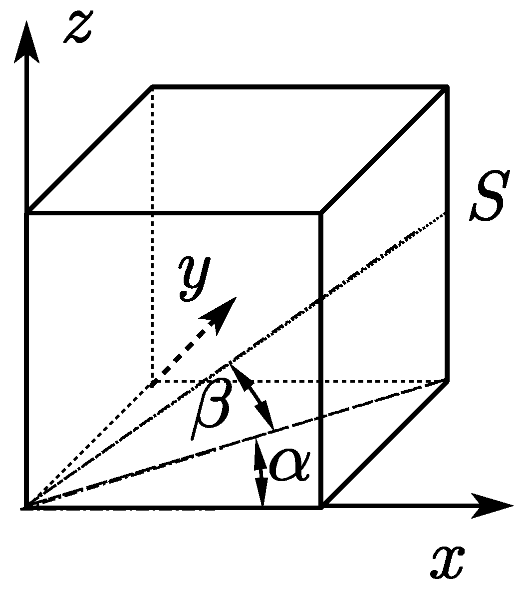
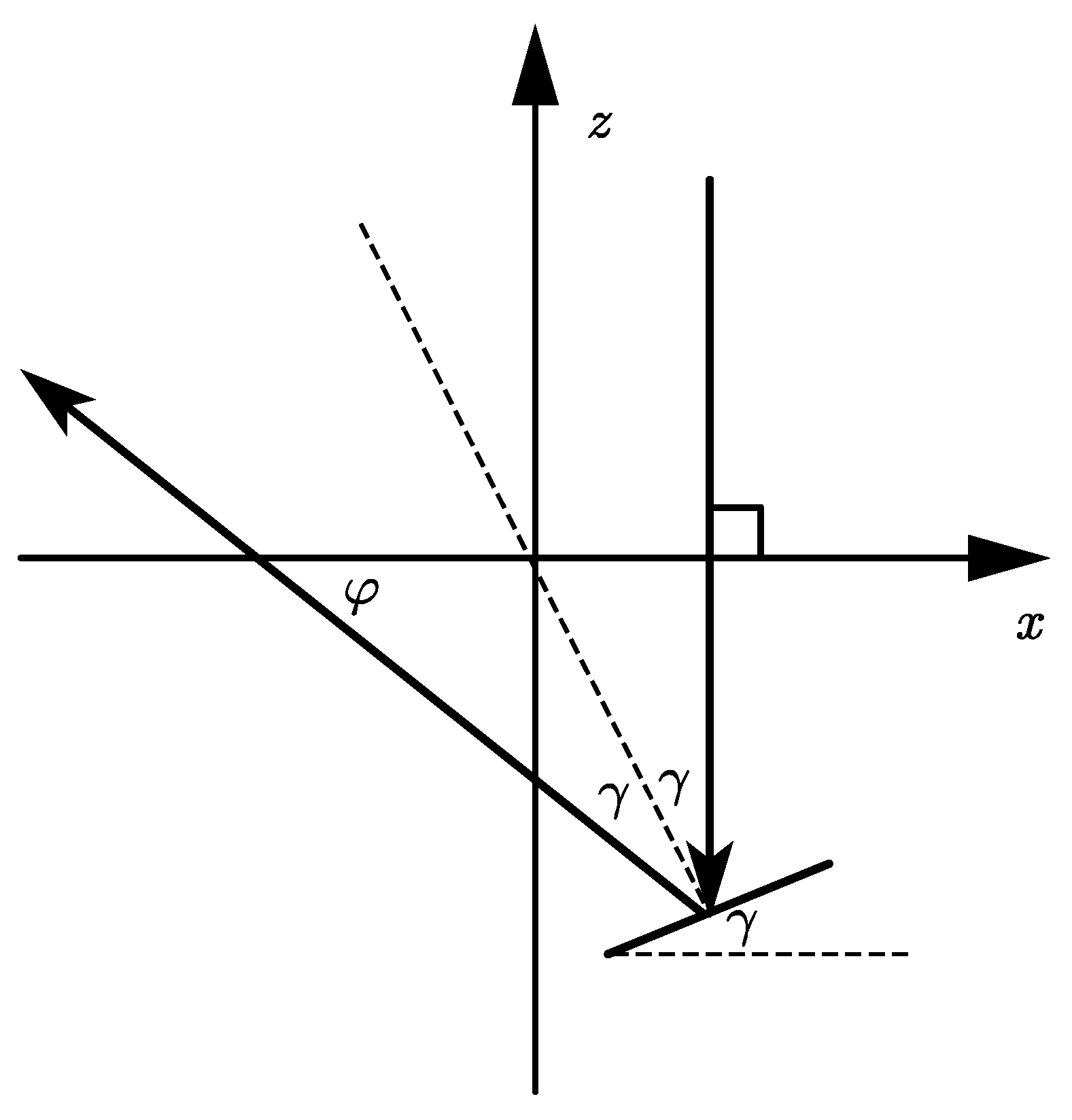
The active reflecting surface of the FAST radio telescope has two forms, namely the datum state and the working state. In the datum state, the reflecting surface is a reference sphere, and all of the main cable nodes are located on it. The radius of the reflecting surface is 300 m, and the aperture is 500 m [13]. The reflecting surface is a paraboloid with an aperture of 300 m in the working state. The sphere radius on which the feed cabin is located is 0.534 times the radius of the datum sphere, and the effective area of the received signal is a disc of radius 0.5 m. The object’s orientation can be determined by azimuth angle $\alpha$ and elevation angle $\beta$. The three-dimensional coordinates were established as seen in Figure 1. Taking the constraints of the reflector panels into account, due to the symmetry of the paraboloid, the ideal working paraboloid was decided when the elevation and azimuth angle of the object to be observed were $\alpha$ = 0° and $\beta$ = 90° respectively.

For a more general case, assuming that the object to be observed is located at $\alpha$ = 36.795°, $\beta$ = 78.169°, an active reflective surface adjustment model was developed to adjust the reflective surface by controlling the radial expansion and contraction of the actuator to bring it close to the defined ideal paraboloid [14]. The adjustment quantities were then calculated. The reception ratio of the feed cabin under the working paraboloid state after adjusting the reflecting panel was calculated and compared to that of the datum-reflecting sphere.

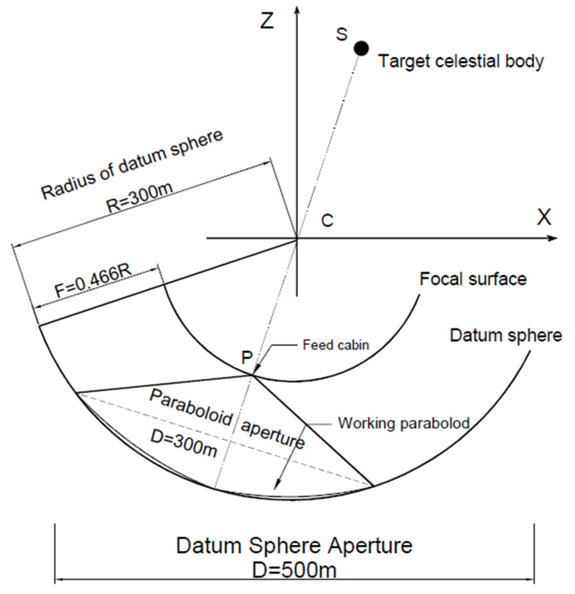
In the case of a three-dimensional coordinate system with the center of the datum sphere as the origin, the ideal working paraboloid and the datum sphere in the same coordinate system are both completely three-dimensional axisymmetrical in all directions, so the problem can be reduced to two dimensions when analyzing the control strategy [15], as shown in Figure 2 below. The main idea is to set the focal length $P/2$ as the optimization variable and to establish a univariate optimization model [16].

Figure 2 is a sectional diagram of the FAST during observation. Point C is the center of the datum sphere. The center of the receiving plane of the feed cabin can only move on one sphere (focal surface) that is concentric with the datum sphere. The radius difference between the two concentric spheres is $F=0.466R$, and R is the radius of the datum sphere. The effective area of the signal received by the feed cabin is a central disk with a diameter of 1 m. When the FAST observes the target celestial body S in a certain direction, the center of the receiving plane of the feed cabin moves to the intersection P of the straight line SC and the focal surface, and part of the reflection panel on the reference sphere are adjusted to form an approximate rotating paraboloid with the straight line SC as the axis of symmetry and P as the focus in order to converge the reflection of the parallel electromagnetic waves from the target celestial body to the effective area of the feed cabin.

2.2. Univariate Optimization Modeling

Since both the datum sphere and the working paraboloid of the FAST radio telescope are symmetrical figures, the solution of the ideal paraboloid in a three-dimensional coordinate system is simplified to the two-dimensional condition so that the equation of the ideal parabola in a two-dimensional coordinate system can be obtained [17]. The equation of the ideal working paraboloid can be calculated by the rotation of the ideal parabola around the z-axis.

The arc of the datum sphere and the ideal parabola in the two-dimensional coordinate system [18] can be expressed as:

$$\{\begin{array}{c}{x}^2+z^2=R^2\\ x^2-2P\cdot z-2P\cdot \left(R-h\right)=0\end{array}$$

(1)

where $h$ is the radial offset of the vertex point corresponding to the ideal parabolola from the datum sphere in a two-dimensional coordinate system [19]. The value of $h$ is positive when it moves to the center of the sphere along the radial direction, and it is negative when it moves away from the center of the sphere along the radial direction. In addition, in the process of the reflectors changing from the datum sphere to the working paraboloid, the outer loop of the aperture of the working paraboloid is always connected to the datum sphere, that is, at the position of $x=\pm D/2$($D$ is the aperture of the paraboloid), Equation system (1) holds. Moreover, since all of the points are located on the negative half axis of the z-axis, the formula for $z$ is expressed as $z=-\sqrt{R^2-x^2}$. Thus, the expression of $h$ can be obtained as seen below:

$$h=R-\sqrt{R^2-{\left(\frac{D}{2}\right)}^2}-\frac{D^2}{8\cdot P}$$

(2)

where $D$ is the aperture of the paraboloid, $R$ is the radius of the datum sphere, and $P/2$ is the focal length.

The relationship between the focal length $P/2$ and the radial offset of the vertex $h$ is found, and then the optimization variable can be converted to $P$ instead of $h$. In the actual calculation, the analytical formula of $P$ is derived from Equation (2), as shown below:

$$P=\frac{D^2}{8\left(R-\sqrt{R^2-{\left(\frac{D}{2}\right)}^2}-h\right)}$$

(3)

Then, the focal–diameter ratio can be defined as:

$$f=\left(P/2\right)/D=P/2D$$

(4)

where $D$ is the aperture of the paraboloid.

Since the edge point of the working paraboloid is continuous with the datum sphere, the x-coordinates and the z-coordinates of the edge points of the datum sphere and the working paraboloid are the same, so the actuators corresponding to the boundary main cable nodes located at the edge points would not expand or contract, and the displacement is 0 [20]. Since the parabola’s focal point is fixed at the focal surface, different parabolas can be obtained by changing the offset $h$ of the vertex. After changing into the working paraboloid, the focal length (i.e., $P/2$) of the corresponding parabola changes from $0.466R$ to $0.466R\pm h$. To establish an objective function that is more realistic, the optimization objective is to minimize the sum of the radial offsets of the points on the ideal parabola from the datum sphere. Since the corresponding central angle of the working paraboloid before adjustment is 60°, assume that some radial lines in the range of 60° are emitted from the center of the circle in the two-dimensional plane, which have an intersection with both the circular arc and the ideal parabola. Thus, the parabola is segmented by these radial lines to simulate the unsmooth situation caused by the fact that the working paraboloid is composed of triangular reflectors.

Using the following system of equations:

$$\{\begin{array}{c}z=\tan \alpha \cdot x\\ x^2-2P\cdot z-2P\cdot \left(R-h\right)=0\\ z^2+x^2=R^2\end{array}$$

(5)

Two kinds of expressions for the horizontal and vertical coordinates of the intersection points on the arc can be found as:

$$x_q\left(i\right)=\{\begin{array}{c}R\cdot \sqrt{\frac{1}{\left({\tan }^2\alpha \left(i\right)+1\right)}}\\ -R\cdot \sqrt{\frac{1}{\left({\tan }^2\alpha \left(i\right)+1\right)}}\end{array}\begin{array}{c}\alpha >\frac{\pi }{2}\\ \alpha \le \frac{\pi }{2}\end{array}$$

(6)

$$z_q\left(i\right)=-\sqrt{R^2-x_q{\left(i\right)}^2}$$

(7)

The two kinds of expressions for the horizontal and vertical coordinates of the intersection points on the parabola can be found as:

$$x_p\left(i\right)=\{\begin{array}{c}\frac{P\cdot {\tan }^2\alpha +\tan \alpha \cdot \sqrt{\left[P\cdot \left(2R-2h+P\cdot {\tan }^2\alpha \right)\right]}}{\tan \alpha }\\ \frac{P\cdot {\tan }^2\alpha -\tan \alpha \cdot \sqrt{\left[P\cdot \left(2R-2h+P\cdot {\tan }^2\alpha \right)\right]}}{\tan \alpha }\end{array}\begin{array}{c}\alpha >\frac{\pi }{2}\\ \alpha \le \frac{\pi }{2}\end{array}$$

(8)

$$z_p\left(i\right)=\frac{\left(x_p^2\left(i\right)-2P\cdot \left(R-h\right)\right)}{2P}$$

(9)

By varying the value of the offset $h$, different parabolas can be obtained. Among these parabolas, the least squares method is used to establish the objective function. The least squares method is used to optimize the sum of the radial offsets of the points on the parabola to be the least, while both the Fibonacci method and the golden mean method are used to search for the optimal solution for $h$ for the sake of accuracy. The objective function is shown below:

$$\min {\displaystyle \sum }_{i=1}^N\sqrt{{\left[x_q\left(i\right)-x_p\left(i\right)\right]}^2+{\left[z_q\left(i\right)-z_p\left(i\right)\right]}^2}$$

(10)

2.3. Modeling of Active Control of Reflective Panels

2.3.1. Determination of the Adjustment Area

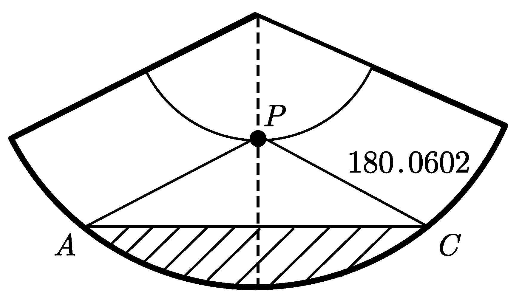
Based on the general case mentioned above, the incident electromagnetic wave is regarded as a ray passing through the origin with the elevation and azimuth angle of $\alpha$ = 36.795°, $\beta$ = 78.169°. As the working parabolic aperture is known to be 300 m, and the ray intersects the focal point with the focal plane, the distance between the boundary point of the ideal paraboloid and the focal point can be calculated, resulting in a distance of 180.0602 m as shown in Figure 3. The main cable nodes whose distance from the focal point is less than this length is the part to be adjusted.

The coordinates of the focal point of an ideal paraboloid are found using the following equation:

$$\{\begin{array}{c}x=-\left(R-0.466R\right)\cdot \cos \beta \cdot \cos \alpha \\ y=-\left(R-0.466R\right)\cdot \cos \beta \cdot \sin \alpha \\ z=-\left(R-0.466R\right)\cdot \sin \beta \end{array}$$

(11)

The coordinates of the vertex of the ideal paraboloid before adjustment are:

$$\{\begin{array}{c}x=-R\cdot \cos \beta \cdot \cos \alpha \\ y=-R\cdot \cos \beta \cdot \sin \alpha \\ z=-R\cdot \sin \beta \end{array}$$

(12)

The coordinates of the vertex of the ideal paraboloid after adjustment are:

$$\{\begin{array}{c}x=-\left(R-h\right)\cdot \cos \beta \cdot \cos \alpha \\ y=-\left(R-h\right)\cdot \cos \beta \cdot \sin \alpha \\ z=-\left(R-h\right)\cdot \sin \beta \end{array}$$

(13)

The critical distance is 180.0602 m. MATLAB software was used to search for the main cable nodes whose distance from the focal point is less than the critical distance so as to determine the nodes that need to be adjusted.

2.3.2. The Two-Dimensional Discrete Actuator Expansion and Contraction Model

For the solution of the actuator expansion and contraction, a two-dimensional discrete actuator expansion and contraction solution model was developed using the idea of discretization. As the corresponding three-dimensional coordinate system has been established and the coordinates of each main cable node are known, the vector formed by the line between the main cable nodes and the sphere center at each end of each main cable was used to calculate the corresponding sphere center angle of all of the main cables [21]. In a coordinate system with the center of the sphere as the origin, let the coordinates of the 2226 principal cable nodes be denoted as $A_i=\left(x_i,y_i,z_i\right),i=1, 2,\dots , 2226$. Then, the spherical center angle between any main cable node and the z-axis can be obtained by the following formulas:

$$\{\begin{array}{c}{A}_i=\left(x_i,y_i,z_i\right)\\ A_{i+1}=\left(x_{i+1},y_{i+1},z_{i+1}\right)\\ \left|A_i\right|=\sqrt{x_i^2+y_i^2+z_i^2}\\ \left|A_{i+1}\right|=\sqrt{x_{i+1}^2+y_{i+1}^2+z_{i+1}^2}\\ \cos \theta =\frac{A_i\cdot A_{i+1}}{\left|A_i\right|\cdot \left|A_{i+1}\right|}\end{array}$$

(14)

Then, obtain:

$${\theta }_j=\arccos \left(\frac{A_i\cdot A_{i+1}}{\left|A_i\right|\cdot \left|A_{i+1}\right|}\right), j=1, 2,\cdots , 6525$$

(15)

Then, the average of all spherical center angles $\overline{\theta }=\left({{\displaystyle \sum }}_{j=1}^{6525}{\theta }_j\right)/6525$, and it can be assumed that the corresponding spherical center angle of every triangular reflector panel is $\overline{\theta }$,which is then used in the two-dimensional simplification as well. Since the corresponding central angle of the two-dimensional working parabola is 60°, the number of segments into which the parabola is divided in the two-dimensional coordinate system by discretization is $N=60°/\overline{\theta }$. Additionally, the number of nodes is $n=N+1$.

Using the model established above for solving the offset of the actuators in the state of the ideal parabola, the central angle 60° is discretized and is divided equally into $N$ parts, and each part has the central angle of $\overline{\theta }$. There is a total of $n$ radial lines used to segment the ideal parabola. For each segment of the discrete parabola, the expansion and contraction of the actuator corresponding to this segment can be calculated later.

The focal coordinates of the ideal paraboloid are obtained from the formula mentioned previously. Using the focal coordinates, find the coordinates of the main cable node closest to the focal point and take it as the vertex of the parabola. This main cable node is then regarded as the base point of the model, which is defined as loop 0. Since the number of segments $N$ of the parabola has already been found, starting from the vertex of the parabola, there are $N/2$ segments for both its left and right sides. The max value among the spherical center angles ${\theta }_j$ is defined as the unit angle. The following loop model could be subsequently built.

2.3.3. The Three-Dimensional Working Paraboloid Loop Model

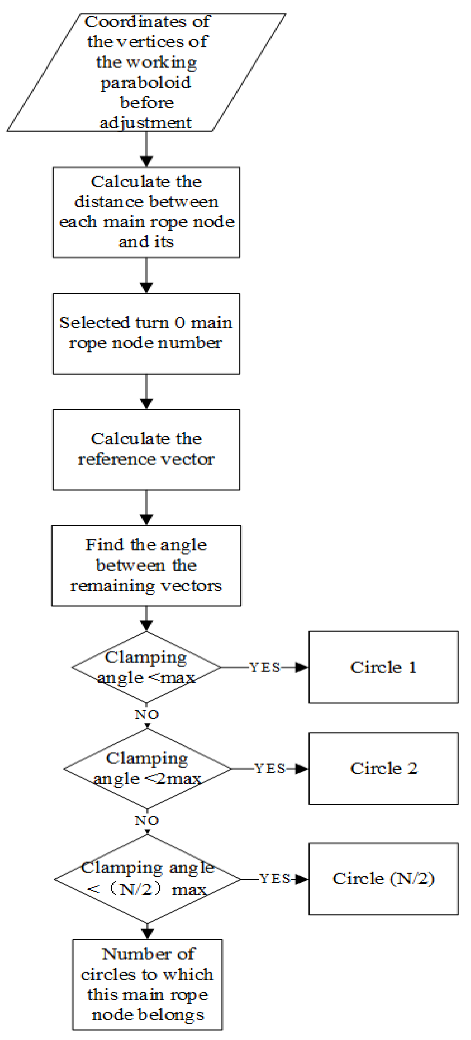
Using the symmetry of the ideal paraboloid, the discretized two-dimensional ideal parabola is rotated around the z-axis to establish the discrete three-dimensional ideal paraboloid model. Thus, there are $N/2$ loops in the working paraboloid in total. The main cable node, which is regarded as the vertex of the idea parabola, is also the vertex of the idea paraboloid, which is defined as loop 0 in this model. The vector formed by the line between the 0-th loop and the center of the sphere is taken as the reference vector. Then, calculate the vectors formed by the connecting line between the other main cable nodes and the spherical center except the main cable node as the parabola vertex. After that, the spherical center angles between the other main cable nodes and the main cable node as the vertex around the spherical center are calculated according to the other vectors and the reference vector. According to the unit angle defined above, it can be determined which loop of the paraboloid each main cable node is located in. Starting from the vertex, the main cable nodes that are i unit angles away from the vertex lie on the i-th loop of the model. Due to the complete symmetry of the paraboloid, it can be considered that the actuators corresponding to the main cable node on each loop in the model has the same offset value. Therefore, the expansion or contraction amount of the actuators calculated in the two-dimensional segment model can be applied to the three-dimensional loop model in order to reasonably simplify the calculation as well as to obtain a more practical estimation value. The flow chart of the calculation process of the loop model is as follows in Figure 4.

As the actuators expand and contract in the radial direction, the main cable nodes also approach or move away from the center of the sphere in the radial direction [22]. The distance between each main cable node and the center of the sphere after adjustment is obtained as ${R_i}^{\prime }=R+h_i$. Using similar triangles, the coordinates of each main cable node after adjustment are calculated as follows:

$$\{\begin{array}{c}{x}_i^{\prime }=\frac{R_i^{\prime }}{R}\cdot x_i=\left(1-\frac{h_i}{R}\right)\cdot x_i\\ y_i^{\prime }=\frac{R_i^{\prime }}{R}\cdot y_i=\left(1-\frac{h_i}{R}\right)\cdot y_i\\ z_i^{\prime }=\frac{R_i^{\prime }}{R}\cdot z_i=\left(1-\frac{h_i}{R}\right)\cdot z_i\end{array}$$

(16)

2.4. Modelling of the Effective Area Reception Ratio of the Feed Cabin

2.4.1. The Model of a Single Triangular Reflective Panel

It was found that the shape of the working paraboloid is fixed in every case due to the symmetry of the working paraboloid, and it is assumed that the triangular reflector panel is uniformly distributed along the surface of the datum sphere [23], so the general incidence problem can be transformed to solve the reception ratio of the feed cabin in the case where the incident light is $\alpha$ = 0°, $\beta$ = 90°. Using the active adjustment model established for the reflective surface, the main cable nodes to be adjusted and the coordinates of these nodes can be obtained after adjustment. Assume that the triangular reflection panel is an equilateral triangle since the coordinates of the three main cable nodes connected to each triangular panel are known, the coordinates of the center of gravity of the triangular reflective panel can be found from the three vertices of the triangle, which can be calculated as follows.

$$\{\begin{array}{c}{x}_0=\frac{x_1+x_2+x_3}{3}\\ y_0=\frac{y_1+y_2+y_3}{3}\\ z_0=\frac{z_1+z_2+z_3}{3}\end{array}$$

(17)

Using the calculated center of gravity coordinates $\left(x_0,y_0,z_0\right)$ to approximate the position of the entire triangular panel. The reflection model for a single triangular reflective panel is represented as follows in Figure 5:

2.4.2. Reflection Validity Judgment Model

It was found that for the same triangular reflective panel, each incident light ray is in the same plane as the reflected ray and that the corresponding elevation angle of the straight line in the same vertical plane is the same. The flow chart of the reflection validity determination model is as follows in Figure 6.

The system of equations are as follows:

$$\{\begin{array}{c}\gamma =\frac{\pi }{2}-\arcsin \left(\left|\frac{z}{R}\right|\right)\\ \varphi =\frac{\pi }{2}-2\gamma \\ \alpha =\arctan \left(\left|\frac{y_0}{x_0}\right|\right)\\ \Delta x=\frac{\Delta z}{\tan \varphi }\cos \alpha \\ \Delta y=\frac{\Delta z}{\tan \varphi }\sin \alpha \end{array}$$

(18)

Equation (18) can be used to determine the number of reflective plates that can effectively reflect the incident light into the plane of the feed cabin, which is denoted as $N_e$. MATLAB software was used to perform a traversal search to find the total number of triangular reflective plates in the working parabolic plane $N_0$. Let the ratio of the reflected signal received in the effective area of the feed cabin to the reflected signal in the working parabolic plane be denoted by $\eta$, then $\eta =\frac{N_e}{N_0}\times 100\%$.

3. Case Study

3.1. Solving the Univariate Optimization Model of the Idea Parabola

The parameters of the ideal paraboloid are easy to find.

The focal points are

$$\{\begin{array}{c}x=-\left(R-0.466R\right)\cdot \cos \beta \cdot \cos \alpha \\ y=-\left(R-0.466R\right)\cdot \cos \beta \cdot \sin \alpha \\ z=-R\cdot \sin \beta \end{array}$$

(19)

In the case of $\alpha$ = 0° and $\beta$ = 90°, the point at the left edge of the aperture: $(-150,-150\sqrt{3})$ and the point at the right edge of the aperture: $(150,-150\sqrt{3})$.

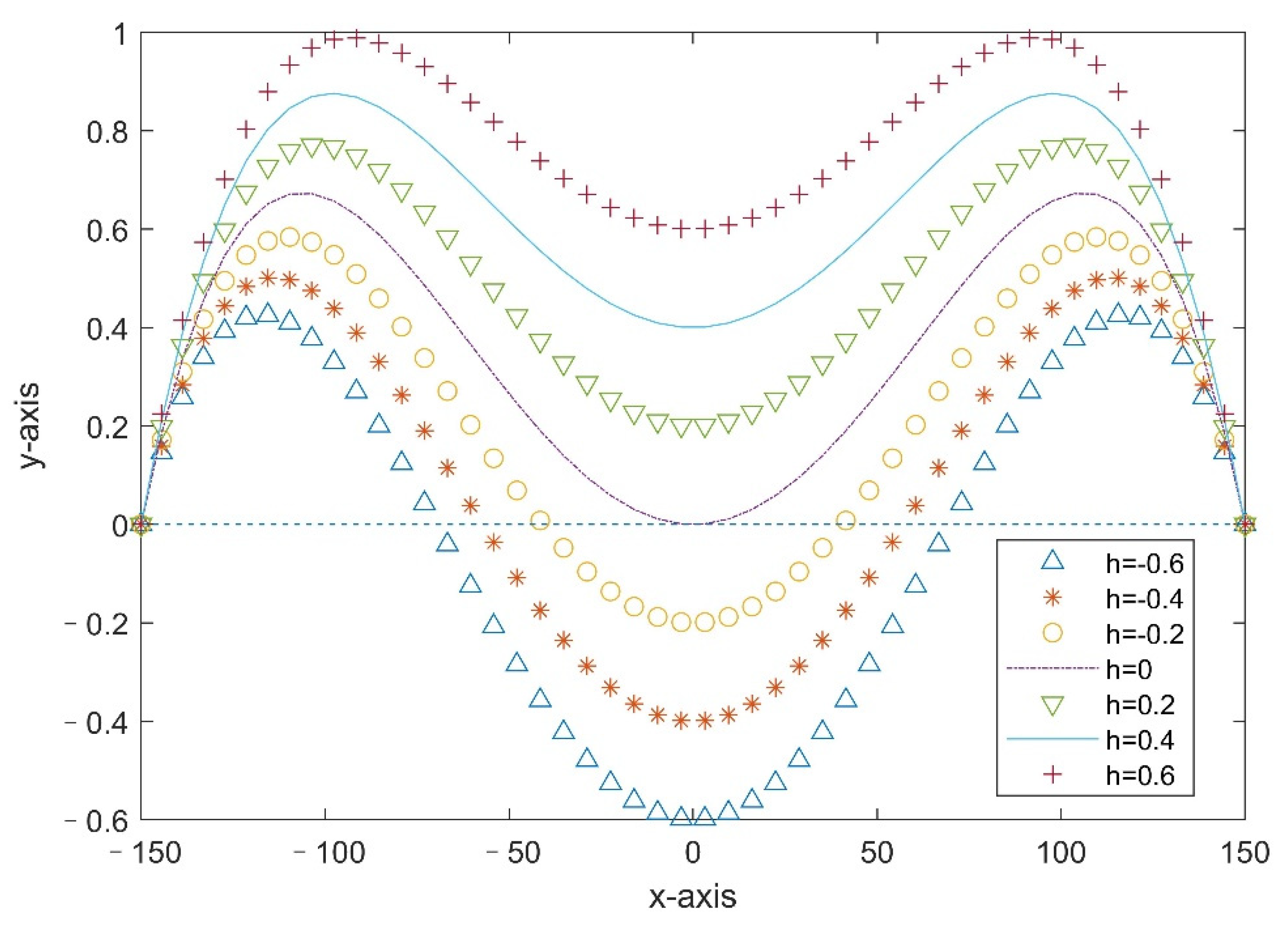
For a different vertex offset $h$, Figure 7 shows the corresponding relationship between the abscissa of each point of the parabola and the radial offset.

Figure 7 shows that the maximum value of the offset in the corresponding ideal parabola is greater than the actuator adjustment limit when $h=-0.4, 0, 0.2, 0.4, 0.6$. Additionally, when $h$ lies between $-0.4$ and $-0.2$, the positive and negative offsets obtained for each point of the ideal parabola are almost equal, that is, the adjusted ideal paraboloid is closer to the original datum sphere to reduce the strain and fatigue of the structure.

It is known that the value of $h$ is between $-0.6$ and $0.6$. On the premise of meeting the optimization objective, the offset reaches the minimum value. The Fibonacci method is then used to search for the radial optimal offset of the ideal parabola vertex $h$, which is $h=-0.33018$ after calculation with the direction that is radially away from the center of the sphere. After that, use the formula $f=\left(\begin{array}{c}0.466R-h\end{array}\right)/D$ to find the focal diameter ratio $f=0.4671$. The golden mean is used to search for the radial optimal offset h as well, which provides the same answer as the Fibonacci method. These two methods are used to search the univariate optimal solution in mathematics, and they only change the search step in different ways. They produce the same answer, which shows that the mathematical model established in this paper has a unique optimal solution.

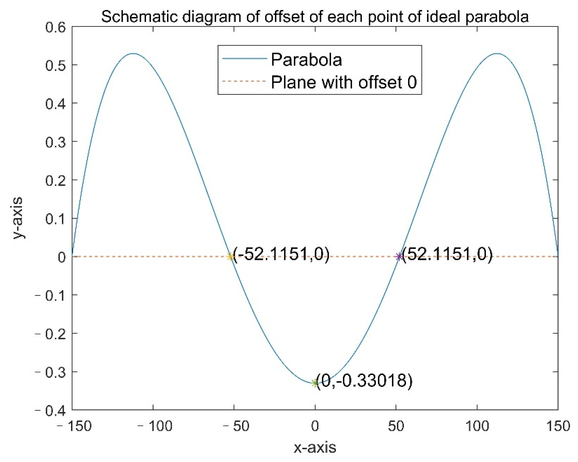
The range of the x-coordinates of the ideal paraboloid is $(-150,150)$. Using the optimal offset h, the focal length of the paraboloid is found using the focal length solution formula $P=\frac{D^2}{8\left(R+\sqrt{R^2-{\left(\frac{D}{2}\right)}^2}-h\right)}$, which, in turn, leads to the ideal paraboloid expression. An image of the radial offset versus the abscissa $x$ at different points on the parabola in a two-dimensional coordinate system should be plotted as follows in Figure 8:

In the ideal parabolic case with $h=-0.33018$ (offset in the direction away from the sphere’s center) and $f=0.4671$, the point with horizontal coordinate $\pm 52.1151$ has an offset of 0, and the maximum offset does not occur at the vertex.

Using the optimal focal length from the single-objective optimization model combined with the boundary conditions and the focal point coordinates, the expression for the ideal paraboloid in the $x-z$ plane can be obtained based Equation (1).

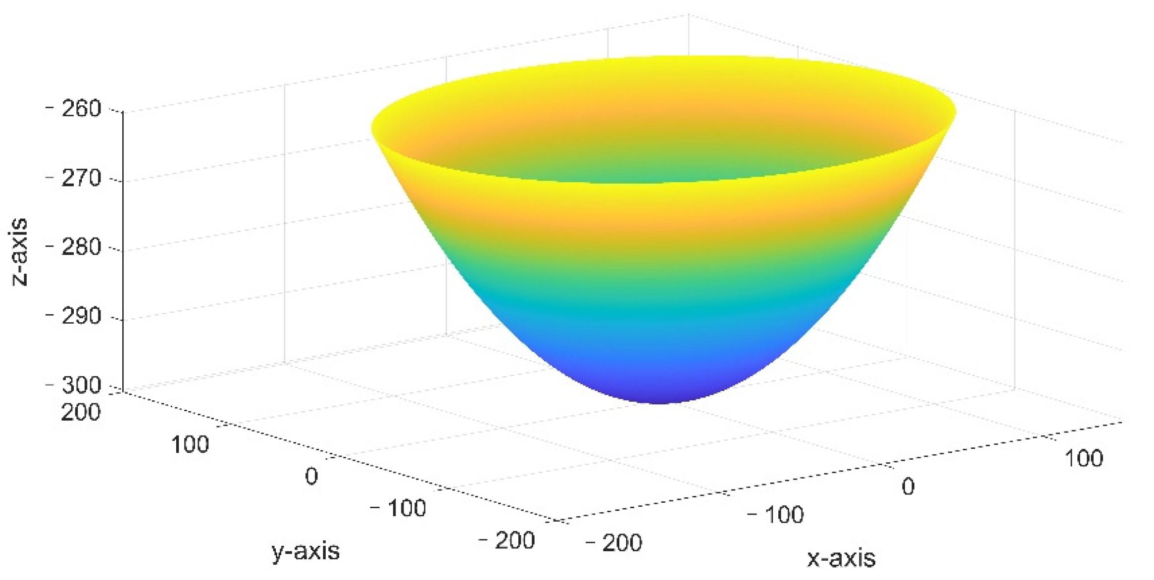
Due to the symmetry of the ideal paraboloid, the 3D figure of the ideal paraboloid can be obtained by rotating the 2D parabola around the z-axis, which is shown in Figure 9.

The equation for the ideal paraboloid is:

$$z=\frac{\left(x^2+y^2\right)}{2P}-\left(R-h\right)$$

(20)

where $P=\frac{D^2}{8\left(R-\sqrt{R^2-{\left(\frac{D}{2}\right)}^2}-h\right)}\left(h=-0.33018,R=D=300\right)$, which is substituted into Equations (20) and (21) and can thus obtain the expressions for the two-dimensional ideal parabola and the three-dimensional ideal paraboloid:

$$x^2-555.25z-166757.2=0$$

(21)

$$z=\frac{\left(x^2+y^2\right)}{555.25}-300.33018$$

(22)

3.2. Solution of the Active Control Model of the Reflective Surface

For a more general calculation case, the elevation and azimuth angle could be $\alpha$ = 36.795°, $\beta$ = 78.169°, respectively. Using the active adjustment model of the reflective surface established before, the number of main cable nodes to be adjusted is calculated as 684. If the incident light enters vertically, that is $\alpha$ = 0°, $\beta$ = 90°, then the number of nodes that need to be adjusted is 706. Combined with the optimal radial offset of the ideal paraboloid of $h=-0.33018$ obtained above, the coordinates of the vertex of the ideal paraboloid could be calculated as $\left(-49.31,-36.88,-293.95\right)$, and $D27$ is determined as the number of main cable node for the 0 loop. The position of the adjusted ideal paraboloid in 3D space is represented in Figure 10.

Using the two-dimensional discrete actuator expansion and contraction model, the following parameters could be acquired: Since the average spherical center angle of the main cable is $\overline{\theta }=0.0379rad$ and the circular center angle of the two-dimensional working parabola is 60°, the number of segments $N=60°/\overline{\theta }=27.6017\approx 28$ and the number of nodes $n=N+1=29$ into which the parabola is divided in the discretized two-dimensional coordinate system are found. This means that in the simulation case established in this paper, taking the vertex of the working paraboloid as the starting point, there are 14 segments to the left and right of the starting point in the two-dimensional parabola, respectively, and each segment simulates a triangular reflector panel, while in the three-dimensional parabola, it is considered that there are 14 loops of triangular reflectors in total. In the two-dimensional coordinate system, the center angle 60° corresponding to the working parabola is discretized and is divided equally into 28 parts. As mentioned earlier, the connecting line between the main cable node as the vertex of the parabola and the sphere center is defined as the reference vector, and the other vectors are the lines formed by the connecting of other main cable nodes and the sphere center. The angle between the reference vector and other vectors is the divergence angle that corresponds to the relevant main cable nodes. For the idea working parabola, the relationship between different divergence angles and the corresponding offset value of the relevant main cable nodes are shown below:

It can be found that this figure is almost symmetrical, which is consistent with the symmetry of an ideal paraboloid. The offset in Figure 11 is the radial displacement value of the main cable nodes, which is also the expansion and contraction value of the actuators in the two-dimensional coordinate system.

Each reflective triangular panel is composed of three main cables and three main cable nodes. There are also three spherical center angles that are formed by connecting the main cable nodes and the sphere center. For the whole reflection surface, it is known that there are $6525$ main cables needed to form the three sides of the triangular reflectors. Through calculations, the range of all the spherical center angles vary from $0.0346rad$ to $0.0413rad$. Based on the three-dimensional working paraboloid loop model established before with the maximum spherical center angle $0.0413rad$, which is the unit angle [24], the number of loops to which each of the main cable nodes belong to can be obtained. It is also considered that in the three-dimensional case, the expansion or contraction amount of the actuators corresponding to the main cable nodes in each loop is the same, then the corresponding radial displacement of all of the main cable nodes that need to be moved can be solved. Finally, the coordinates of each of the main cable nodes after adjustment can be obtained using similar triangles.

The working paraboloid formed after the adjustment of the datum sphere and the three-dimensional projection of the original datum sphere to the $x-z$ plane are as follows in Figure 12:

The trasversal search in MATLAB shows that with the total number of triangular reflective panels $N_0=1325$, the corresponding main cable node number can also be determined. After active adjustment, the coordinates of the center of gravity of each triangular reflector panel could all be calculated. Using the reflection validity judgment model to determine the number of valid triangular reflective panels out of 1325, that is $N_e=125$, then $\eta =\frac{N_e}{N_0}\times 100\%=9.434\%$.

3.3. Solution of a Baseline Reflective Spherical Simulation Model

Calculate the reception ratio of the reference reflecting sphere for a hypothetical incident light line $\alpha =36.795°, \beta =78.169°$, i.e., the ratio of the reflected signal received in the effective area of the feeder compartment to the reflected signal from the reference sphere within a 500 m aperture. Since the electromagnetic wave signal propagates in a straight line parallel to the visible light propagation law, it was idealized by replacing the electromagnetic wave signal with a light beam in the LightTools optical system modelling software.

Firstly, during the modelling of the reference spherical reflecting sphere, a reflector with a radius of 300 m and an aperture of 500 m was selected as the active reflecting panel of the reference sphere.

During the modelling of the parallel electromagnetic wave source, the surface light source was selected as the base component. The light path was set to the positioning area. The angle distribution was set to uniform. The tracing direction was adjusted outward, and the positioning angle of the positioning sphere was 0° both up and down to achieve the setting of the parallel electromagnetic wave source. The practical receiving area of the feeder compartment was then set to accommodate the receiver with a dimensional radius 0.5 m, thus establishing an ideal reflective spherical light simulation model.

It is also known that the effective receiving area of the feeder compartment is parallel to the emission plane of the parallel electromagnetic wave source, so the plane $B$ is parallel to the above two planes. With $\alpha$ and $\beta$ known, let the angle of plane $B$ to the x-axis be $\Omega$, the angle to the y-axis be $\Psi$, and the distance from the origin where the center of the sphere is located be $OB$. From the knowledge of three-dimensional geometry to find the angle between a line and a plane in space, it follows that:

$$\{\begin{array}{c}\Omega =\arccos \beta \cdot \cos \alpha \\ \Psi =\arccos \beta \cdot \sin \alpha \end{array}$$

(23)

Substitute $\alpha =36.795°, \beta =78.169°$ and obtain:

$$\{\begin{array}{c}\Omega =9.45°\\ \Psi =7.1128°\end{array}$$

(24)

The angle between plane B and the z-axis is also easily obtained as A. Therefore, the effective receiving area of the feeder module is found to be in the plane and the azimuth of the parallel electromagnetic wave source emission plane. Subsequently, according to the spatial geometry relationship, the $x, y, z$ coordinate expression of the feeder module is determined to be

$$\{\begin{array}{c}x=0.534R\cdot \cos \beta \cdot \cos \alpha \\ y=0.534R\cdot \cos \beta \cdot \sin \alpha \\ z=0.534R\cdot \sin \beta \end{array}$$

(25)

Substitute to obtain $x=26.3018, y=19.6727, z=156.7968$. The distance between the emitting surface of the parallel electromagnetic wave source and the origin of the sphere center is set to 50 m to obtain $x=8.209, y=6.140, z=48.937$. The actual size is also scaled to $10000:1$ in the simulation software.

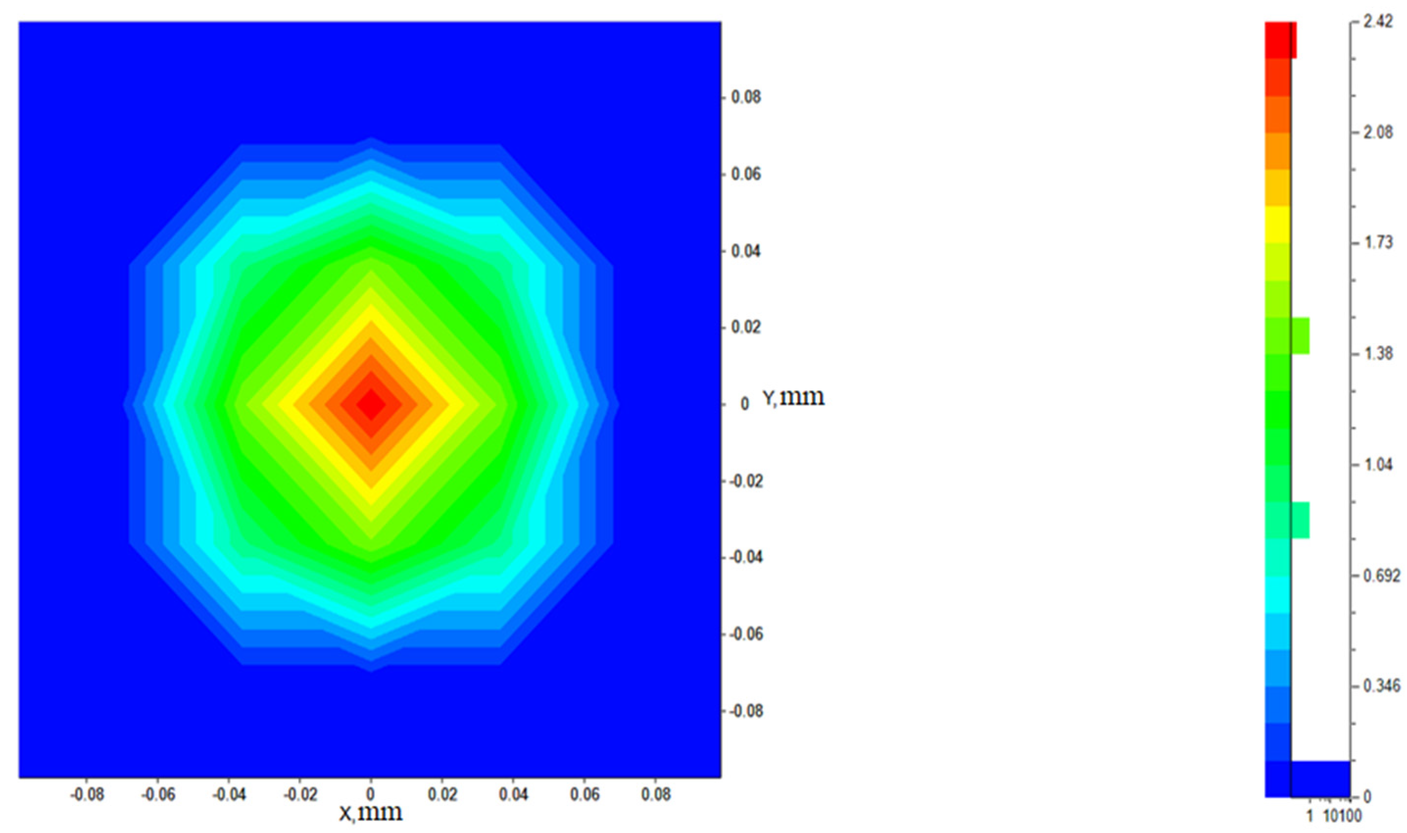
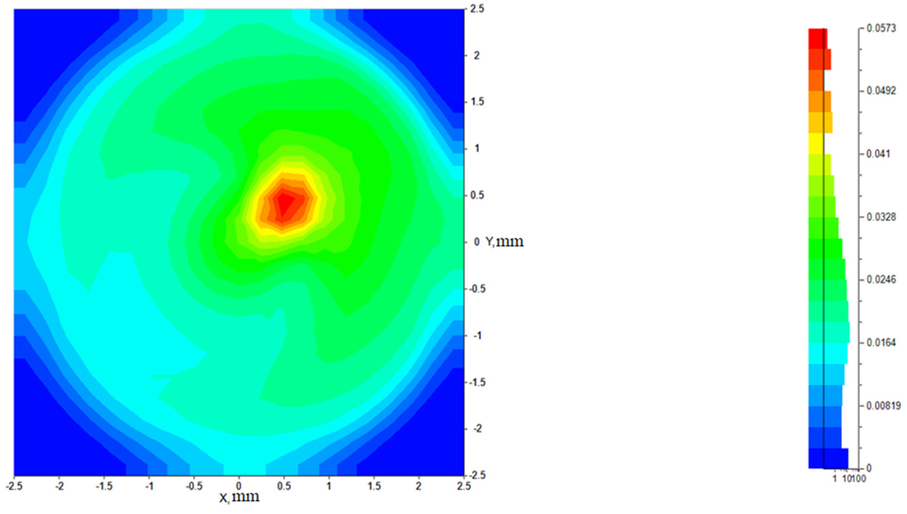
Finally, the total number of rays to be traced was set to 25 million in the simulation input to perform the ray tracing simulation. The simulation is illustrated below. On the left is a diagram where the rendering mode is transparent, and on the right is a diagram with the intensity displayed. As the default reflective sphere needs to be built on a cylinder, a sphere is cut out of the top surface of the cylinder to simulate the main reflective surface, and an opaque material is applied to the surface of the cylinder.

LumViewer illuminance analysis of the effective receiving area of the feeder compartment shows that the total number of reflected rays received in the effective area of the feeder compartment is 183,370, and the spherical reflective surface with the surface receiver set as the receiving area for illuminance analysis shows that the total number of reflected rays in the reference sphere is 13,193,834. Figure 13 shows the received intensity of the reference sphere and the color of the diagram from blue to red, representing the increasing intensity. The final ratio of the base reflecting sphere is $1.3898\%$.

Compared to the working paraboloid acceptance ratio $9.434\%$ found above, the working paraboloid acceptance ratio is expanded by a factor of almost seven. Figure 14 and Figure 15 show the reception strength in the effective area of the deed cabin and datum sphere respectively.

3.4. Analysis of Structural Fatigue Damage Problems

Under the discrete loop model developed in this paper, it is considered that the expansion or contraction of each node lying on the same loop is equal to each other from the 1st loop to the 14th loop. However, the actual situation is more complex [25]. The constant transformation between the datum paraboloid and the working paraboloid results in a constant change in the distance between the main cable nodes. When the strain of the main cable exceeds a certain value, generally assumed to be $0.17~0.18\%$, the reflective panel is in a fatigue working condition and the main cable network is at risk of fracture.

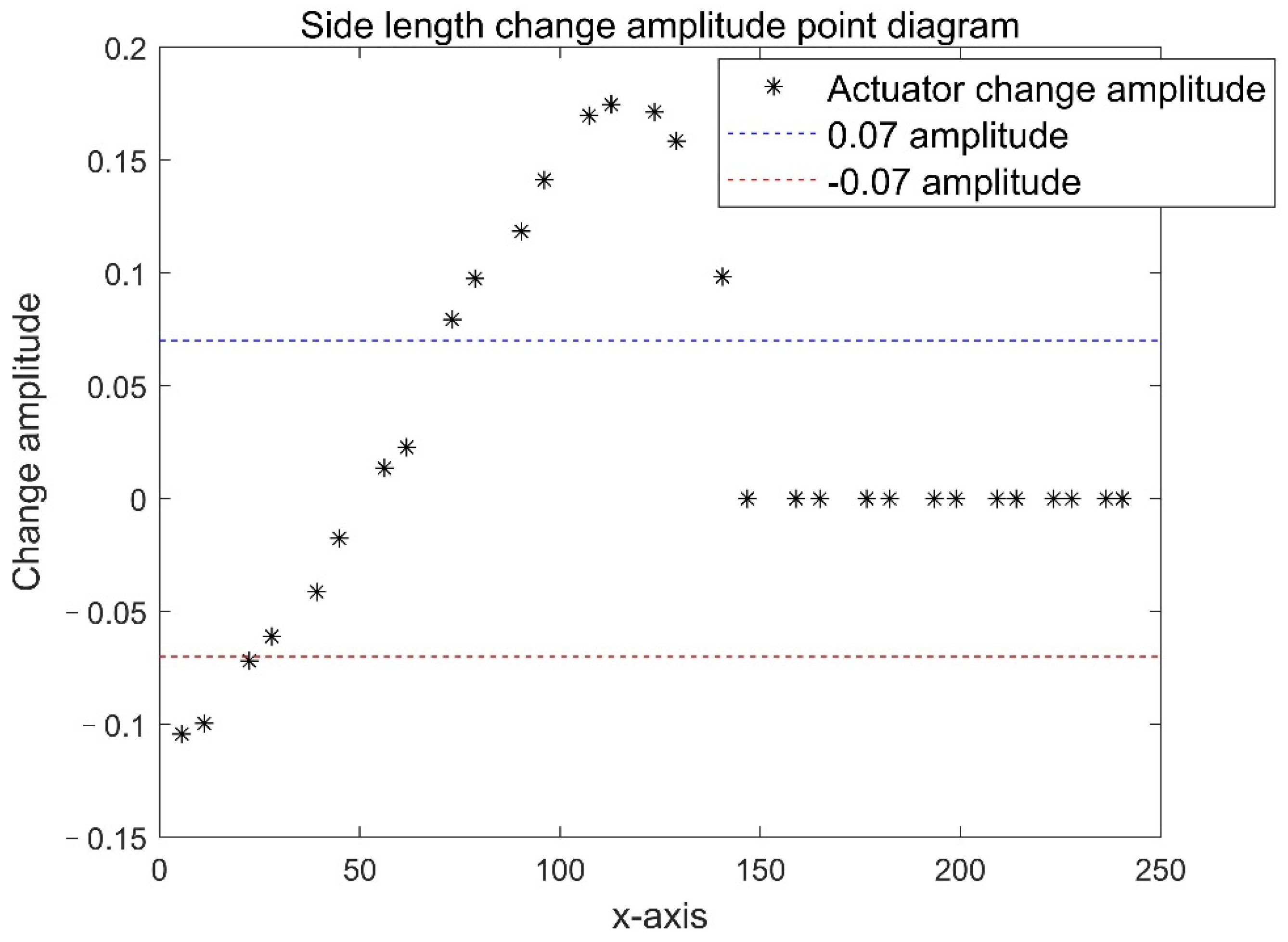
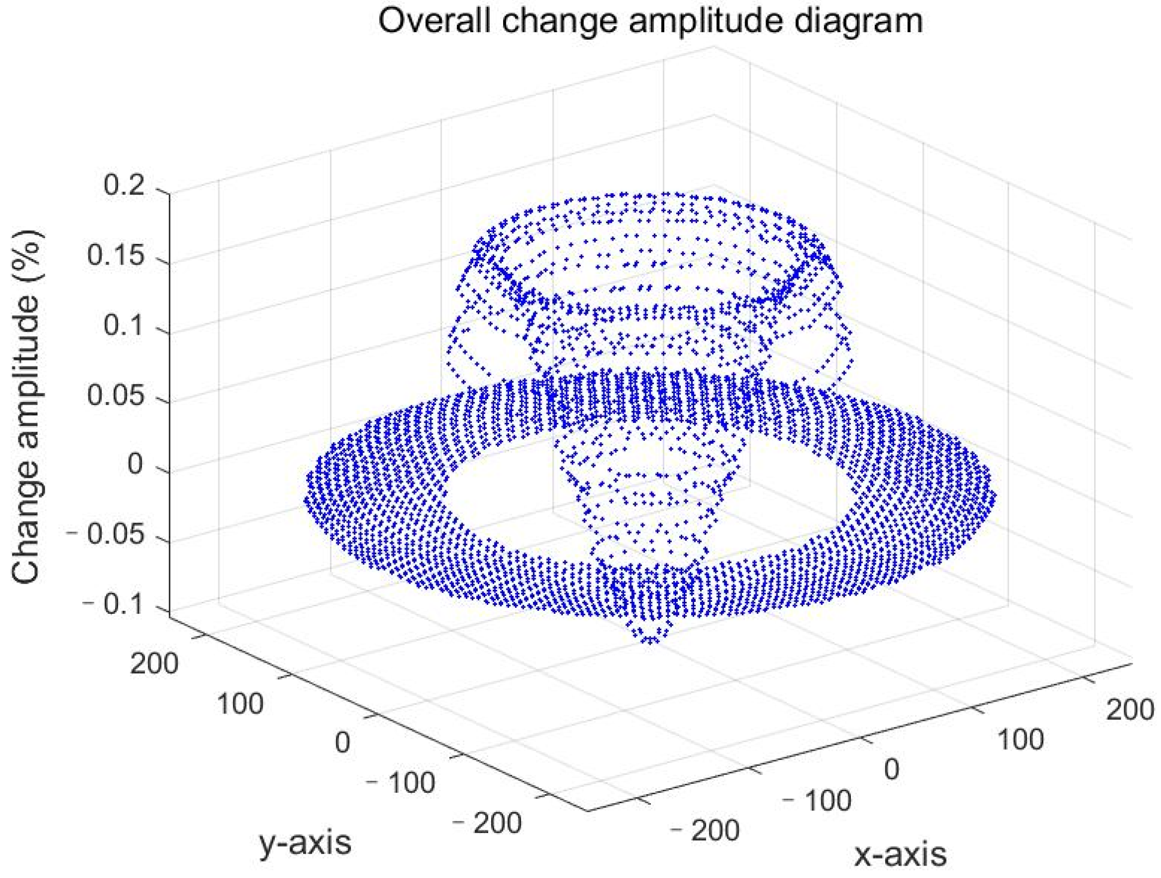
From the previous calculation results, the distance change amplitude of each node first becomes smaller and then larger and finally smaller, where a few points elongate up to $0.1746\%$. However, the overall compression is only $0.1042\%$ at most, the length change amplitude is not significant, only $15.6\%$ experience a length change amplitude up to $0.17\%$, and no length change amplitude exceeds 0.715%, i.e., there is a risk of fracture for very few main cables. The two-dimensional diagram shows that the spacing of the adjacent nodes near the outermost loop may show large variation and may require special reinforcement treatment, which is shown in Figure 16. Moreover, the three-dimensional diagram in Figure 17 shows that the changed triangular plate basically conforms to the shape of the ideal paraboloid, which shows that the simulation of the model established in this paper is superior.

4. Discussion

4.1. Advantages of the Model

• The univariate optimization model established here aims to minimize the radial offset between the ideal paraboloid and the reference paraboloid. Compared to some studies in the literature that only calculate the vertical offset, the radial offset calculated in this paper is more in line with the actual situation. The vertical offset refers to the displacement of the active reflecting surface in the vertical direction. However, in practice, the reflecting panel can only move along the radial direction, and the included angle between the moving direction and the horizontal plane is $\theta =\arccos \left(\frac{\left|Z\right|}{R}\right)$. Therefore, only considering the vertical displacement will ignore the horizontal displacement, that is $R\cos \left(\theta \right)$, resulting in a deviation from the actual results.
• In the univariate optimization model, the optimization variable is the vertex offset of the ideal paraboloid, and the Fibonacci method and golden section method are used to search for the optimal solution. The optimal solution obtained by the two methods is $h=-0.33018$, and the error is less than ${10}^{-5}$, and the accuracy is high.
• The active adjustment model of the reflective panel is established using the idea of the discretization, the expansion, and contraction of each main cable node in the two-dimensional case. Then, the working paraboloid was divided into 14 loops by using the working paraboloid loop model, and then the expansion and contraction in the three-dimensional case was obtained. This model considers the non-smoothness of the active reflection panel, and the calculation results are more in line with the actual situation. After adjustment, the receiving ratio of the active reflection panel increased from 1.3898% in the reference state to 9.434% in the working state, which is 6.8 times that of the original.
• In the established reflection effectiveness judgment model, the actual situation of the working paraboloid was considered when calculating the reception ratio, that is, the non-smoothness of the reflecting surface was not ignored, and the working paraboloid was discretized into 1325 triangular reflection panels, which is more appropriate to the actual situation than directly calculating the reception ratio with the smooth ideal paraboloid.
• In this paper, the optical system modelling software LightTools was used to model the datum sphere to calculate the effective receiving ratio, which was 1.3898%, which provides some reliable data for latecomers.

4.2. Aspects That Need Further Study

When calculating the reflected signal from the working paraboloid, the effect of the feed cabin on the incident EM wave signal was not considered and may somewhat bias the results.

4.3. Generalization of the Model

FAST is a huge project that contributes to the development and application of astronomy [26]. The active adjustment model of the reflector panel provided in the paper considers the minimum radial offset, the non-smoothness of the datum sphere, and the working paraboloid and uses the idea of discretization. The results obtained here are of great reference value for the active control of the main reflecting surface of the FAST radio telescope. This paper also uses the LightTools optical system modelling software to make the results more intuitive.

The active adjustment model for the reflector proposed in this paper has important reference value for the radio telescope, as it uses active reflector technology. By only inputting the relevant dimensions and constraints of the radio telescope, the adjustment scheme of each actuator of the active reflector and the working paraboloid equation can be output.

References

- Zhang, T. Creation and application of digital twin model for the Five Hundred Meter Spherical Radio Telescope (FAST). Eng. Technol. II 2020, 3, 154–196. (In Chinese) [Google Scholar]
- Li, W.; Zhou, L. A preliminary study on photogrammetry for the FAST main reflector measurement. Res. Astron. Astrophys. 2021, 21, 156–164. [Google Scholar] [CrossRef]
- Nan, R.; Li, H. Progress of FAST—Science, technology and equipment. Chin. Sci. Phys. Mech. Astron. 2014, 44, 1063–1074. [Google Scholar] [CrossRef]
- Li, Q.; Jiang, P.; Nan, R. Design and analysis of the adaptive connection mechanism of the 500 m aperture radio telescope cable network and panel unit. J. Mech. Eng. 2017, 53, 62–68. [Google Scholar] [CrossRef]
- Chen, R.; Zhang, H.; Jin, C.; Gao, Z.; Zhu, Y.; Zhu, K.; Jiang, P.; Yue, Y.; Lu, J.; Zhang, B.; et al. FAST VLBI: Current status and future plans. Res. Astron. Astrophys. 2020, 20, 74–80. [Google Scholar] [CrossRef]
- Zhu, Z.; Liu, F.; Zhang, L.; Wang, Z.; Liang, C.; Xue, Y.; Bai, G.; Deng, X. Primary supporting structure design of Five-hundred-meter Aperture Spherical Telescope (FAST). Space Struct. 2017, 23, 4–8. (In Chinese) [Google Scholar]
- Chen, Y.; Liu, W.; Zhang, Z.; Zhang, T. SETI strategy with FAST fractality. Res. Astron. Astrophys. 2021, 21, 178–185. [Google Scholar] [CrossRef]
- Jiang, P.; Shen, Z.; Xu, R. Preface: Key technologies for enhancing the performance of FAST. Res. Astron. Astro-Phys. 2020, 20, 63–65. [Google Scholar] [CrossRef]
- Kong, X.; Wang, Q. Research on Construction Process of the Cable-net Structure of FAST. IOP Conf. Ser. Mater. Sci. Eng. 2019, 521, 12006. [Google Scholar] [CrossRef]
- Li, D.; Dickey, J.M.; Liu, S. Preface: Planning the scientific applications of the Five-hundred-meter Aperture Spherical radio Tele-scope. Res. Astron. Astrophys. 2019, 19, 16–18. [Google Scholar] [CrossRef] [Green Version]
- Li, H.; Jiang, P. An open-loop control algorithm of the active reflector system of FAST. Res. Astron. Astrophys. 2020, 20, 65–74. [Google Scholar] [CrossRef]
- Li, Q.; Jiang, P.; Li, H. Prognostics and health management of FAST cable-net structure based on digital twin technology. Res. Astron. Astrophys. 2020, 20, 67–75. [Google Scholar] [CrossRef]
- Li, J.; Peng, B.; Jin, C.; Li, H.; Strom, R.G.; Liu, B.; Chai, X.; Liu, L. Adapting active reflector technology for greater sensitivity and sky-coverage in FAST-like telescopes. Mon. Not. R. Astron. Soc. 2021, 501, 6210–6214. [Google Scholar] [CrossRef]
- Li, J.; Peng, B.; Chai, X. Fast lighting aperture analysis. Astron. Res. Technol. 2021, 3, 301–306. [Google Scholar]
- Wang, Z. Research on the Control. Strategy of FAST Whole Network Based on Iterative Learning Theory; Northeastern University: Shenyang, China, 2015. [Google Scholar]
- Jiang, Q.; Xie, J.; Ye, J. Mathematical Modeling, 4th ed.; Higher Education Press: Beijing, China, 2016. [Google Scholar]
- Lv, N.; Wu, D.; Cao, H.; Yang, L.; Fan, J. Deformation Localization of Reflector Antenna Based on Focal-Field Distribution with CapsNet. In Proceedings of the 2020 IEEE International Symposium on Antennas and Propagation and North American Radio Science Meeting, Montreal, QC, Canada, 17 February 2021; pp. 385–386. [Google Scholar]
- Li, M.; Zhu, L. Optimization analysis of FAST transient paraboloidal deformation strategy. J. Guizhou Univ. 2012, 29, 24–28. [Google Scholar]
- Li, J.; Peng, B.; Chai, X. Re-investigation of the Illuminated Aperture of the FAST. Astron. Res. Technol. 2021, 18, 301–306. [Google Scholar]
- Peng, J.; Cao, H.; Wu, D.; Sun, Z.; Fan, J. A Novel Method of Surface Damage Localization for FAST Active-reflector. In Proceedings of the 2020 IEEE International Symposium on Antennas and Propagation and North American Radio Science Meeting, Montreal, QC, Canada, 17 February 2021; pp. 705–706. [Google Scholar]
- Song, L.; Jiang, P.; Wang, Q.; Yang, L. Research on key technologies for installation and maintenance of reflector of FAST. Res. Astron. Astrophys. 2020, 20, 66–72. [Google Scholar] [CrossRef]
- Tang, W.; Zhu, L.; Wang, Q. Recognition of FAST reflector nodes based on Canny operator. Res. Astron. Astro-Phys. 2020, 20, 126–133. [Google Scholar] [CrossRef]
- Yao, R.; Jiang, P.; Sun, J.; Yu, D.; Sun, C. A motion planning algorithm for the feed support system of FAST. Res. Astron. Astrophys. 2020, 20, 68–78. [Google Scholar] [CrossRef]
- Yin, J.; Jiang, P.; Yao, R. An approximately analytical solution method for the cable-driven parallel robot in FAST. Res. Astron. Astrophys. 2021, 21, 46–60. [Google Scholar] [CrossRef]
- Yu, N.; Qian, L.; Zhang, C.; Jiang, P.; Xu, J.; Wang, J. HI detection of J030417.78+002827.4 by the Five-hundred-meter Aperture Spherical Radio Telescope. Res. Astron. Astrophys. 2021, 21, 100–105. [Google Scholar] [CrossRef]
- Zhao, Z.; Liu, M.; Song, L.; Wen, J.; Zhao, W.; Peng, Y. Creation of a digital model of the radio telescope feeder module. Mod. Comput. 2019, 26, 12. [Google Scholar]
Figure 1.
Diagram of azimuth and elevation angles for astronomical observations.
Figure 2.
Schematic diagram of the overall system in two dimensions.
Figure 3.
Schematic representation of the principle of determining the adjustment area.
Figure 4.
Flow chart of the split circle model.
Figure 5.
Plan view of a single triangular reflective panel.
Figure 6.
Flowchart of the reflective validity determination model.
Figure 7.
Corresponding positive and negative offsets of the parabolic points at different focal lengths.
Figure 8.
Offsets at points on an ideal parabola.
Figure 9.
Ideal paraboloid 3D model.
Figure 10.
Schematic diagram of the changed parabola and datum sphere.
Figure 11.
Offsets corresponding to different divergence angles.
Figure 12.
Comparison of plane projections before (A) and after (B) main cable node mesh adjustment.
Figure 13.
Schematic of Light Tools datum sphere simulation.
Figure 14.
Schematic representation of the reception strength in the effective area of the feed cabin.
Figure 15.
Schematic diagram of the datum sphere reception strength.
Figure 16.
Point diagram of the magnitude of change in the edge length of the section.
Figure 17.
Variation of distance between any adjacent main cable nodes before and after adjustment.
Publisher’s Note: MDPI stays neutral with regard to jurisdictional claims in published maps and institutional affiliations. |
© 2022 by the authors. Licensee MDPI, Basel, Switzerland. This article is an open access article distributed under the terms and conditions of the Creative Commons Attribution (CC BY) license (https://creativecommons.org/licenses/by/4.0/).
Share and Cite
MDPI and ACS Style
Wang, Y.; Xiong, Y.; Hao, J.; He, J.; Liu, Y.; He, X. Active Control Model for the “FAST” Reflecting Surface Based on Discrete Methods. Symmetry 2022, 14, 252. https://doi.org/10.3390/sym14020252
AMA Style
Wang Y, Xiong Y, Hao J, He J, Liu Y, He X. Active Control Model for the “FAST” Reflecting Surface Based on Discrete Methods. Symmetry. 2022; 14(2):252. https://doi.org/10.3390/sym14020252
Chicago/Turabian StyleWang, Yanbo, Yingchang Xiong, Jianming Hao, Jiaqi He, Yuchi Liu, and Xinpeng He. 2022. "Active Control Model for the “FAST” Reflecting Surface Based on Discrete Methods" Symmetry 14, no. 2: 252. https://doi.org/10.3390/sym14020252
Note that from the first issue of 2016, this journal uses article numbers instead of page numbers. See further details here.